16 Visualising phylogenies
- Visualize and annotate your tree with
Microreact.
There are many programs that can be used to visualise phylogenetic trees. Some of the popular programs include FigTree, iTOL and the R library ggtree. For this course, we’re going to use the web-based tool Microreact as it allows users to interactively manipulate the tree, add metadata and generate other plots including maps and histograms of metadata variables in a single interface.
In order to use this platform you will first need to create an account (or sign-in through your existing Google, Facebook or Twitter).
16.1 Uploading tree files and metadata
Once you’ve logged into Microreact, you can upload the rooted Namibian TB tree file (Nam_TB_rooted.treefile) and combined metadata TSV file (TB_metadata.tsv) we created earlier.
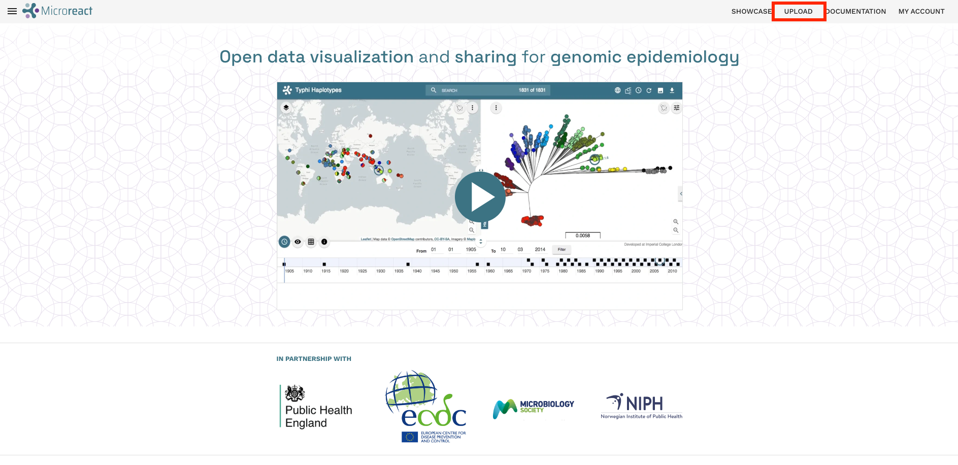
- Click on the UPLOAD link in the top-right corner of the page:
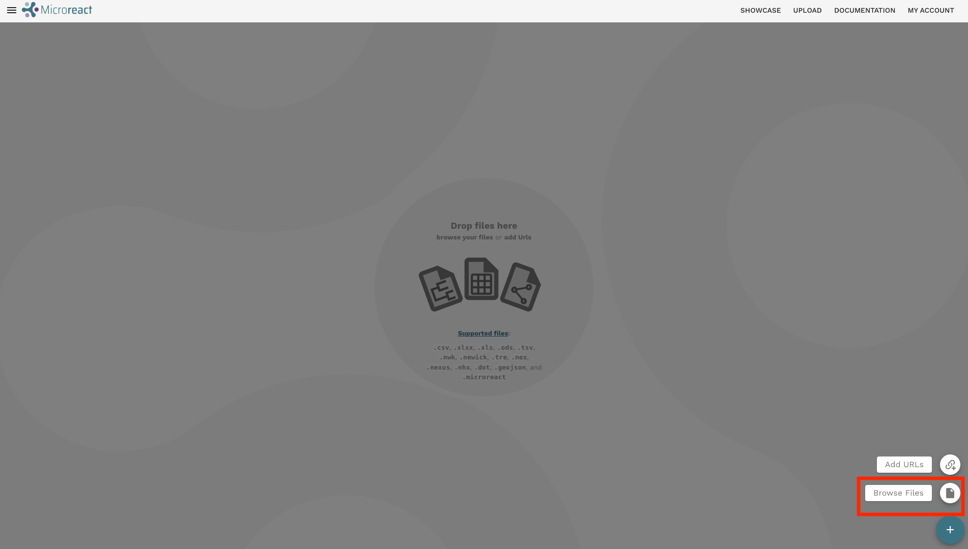
- Click the + button on the bottom-right corner then Browse Files to upload the files:
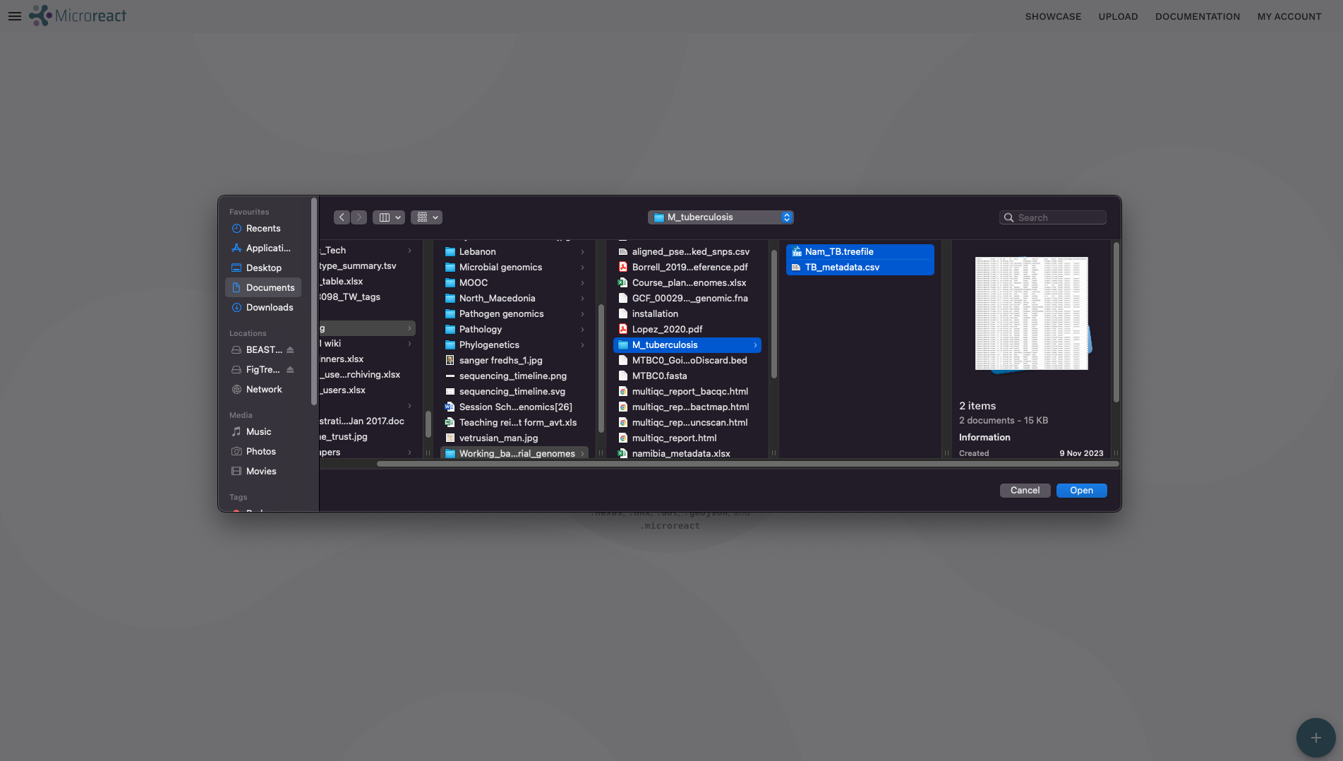
- This will open a file browser, where you can select the tree file and metadata from your local machine. Go to the
M_tuberculosisdirectory where you have the results we’ve generated so far this week. Click and select theNam_TB_rooted.treefileandTB_metadata.tsvfiles while holding the Ctrl key. Click Open on the dialogue window after you have selected both files.
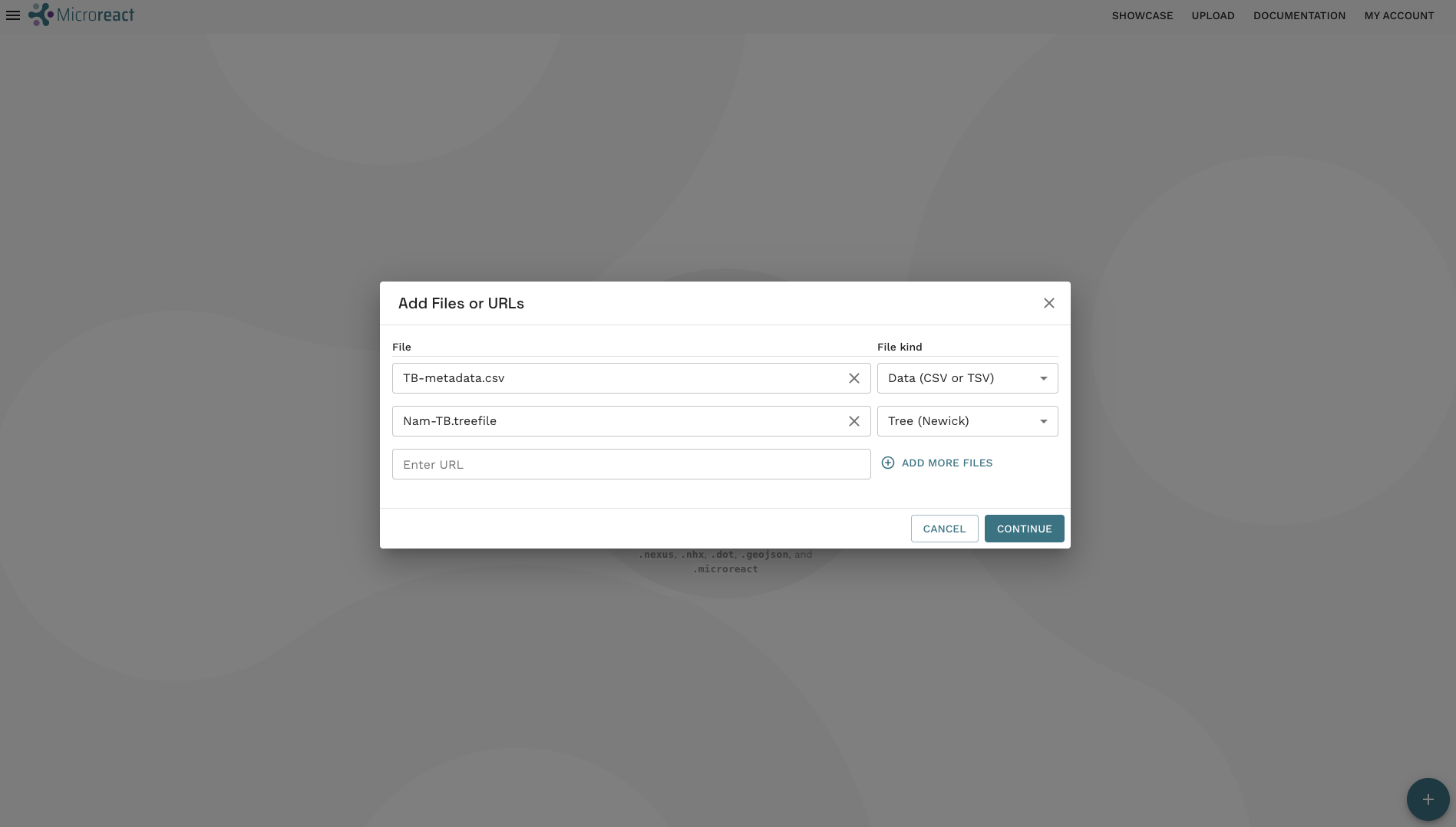
- A new dialogue box will open with files you’ve uploaded and the File kind which is done automatically by Microreact. As the File kind for both files is correct, go ahead and click CONTINUE:
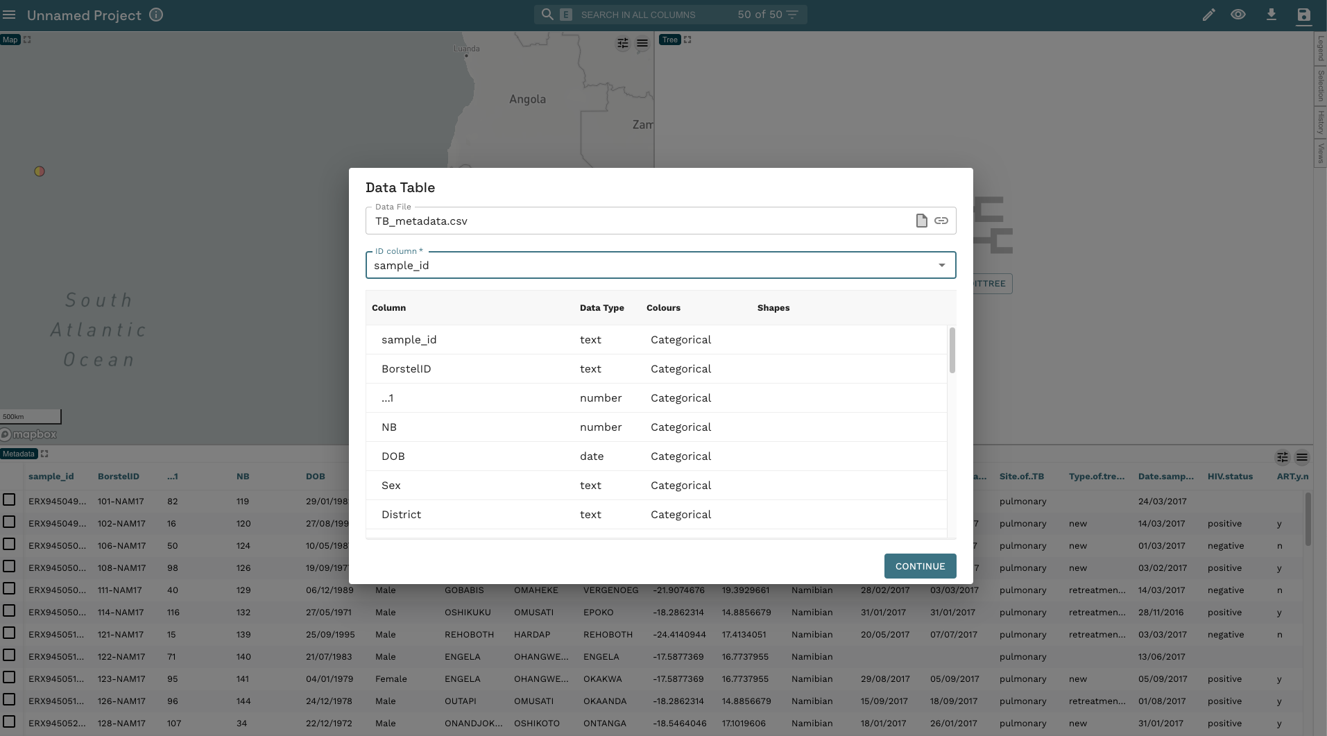
- Microreact will load the data and process it. The final step before we can have a look at the tree and annotate it is to confirm to Microreact which column in the metadata corresponds to the tip labels in the tree so it can match them. By default Microreact will use the first column, in this case
samplewhich is correct so click CONTINUE:
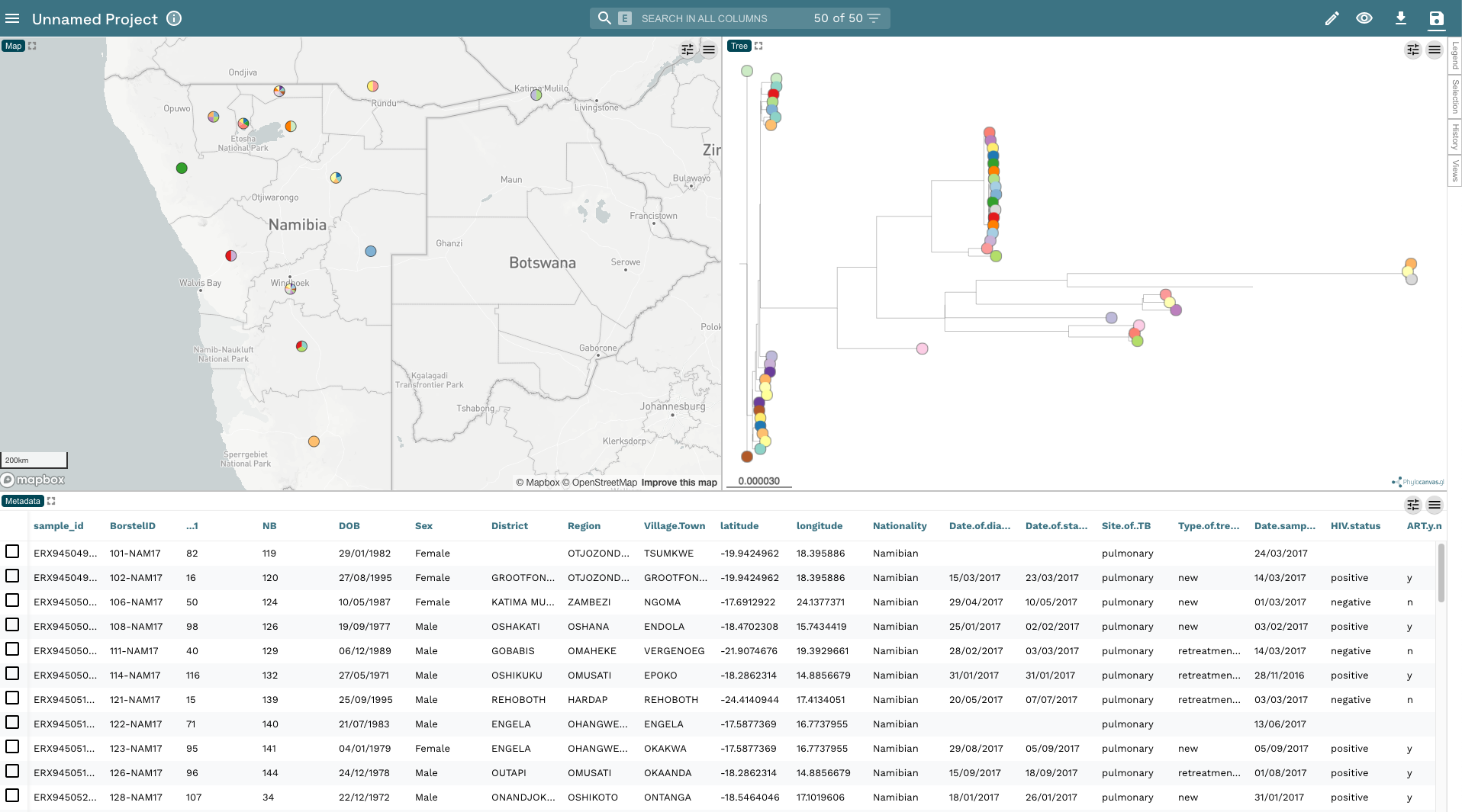
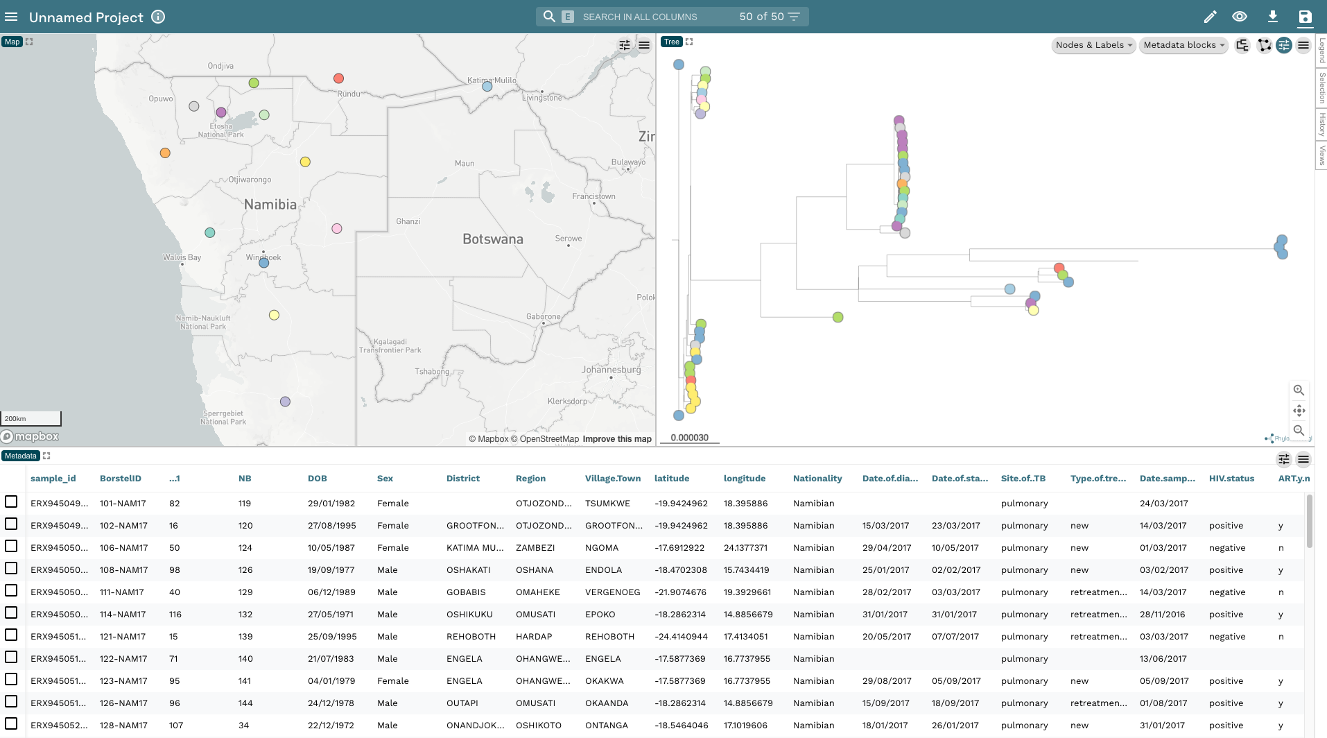
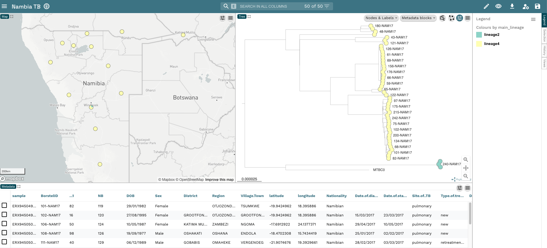
- You should now see three windows in front of you. The top-left has a map with the locations of your isolates based on the longitude and latitude values included in
TB_metadata.tsv. The top-right has the phylogenetic tree with a separate colour for each tip (by default Microreact will colour the tips byBorstelID). Across the bottom you have the metadata fromTB_metadata.tsv.
- The first thing we’re going to do is change the colour of the tip nodes to Region. Click on the Eye icon in the top-right hand corner and change Colour Column to Region:
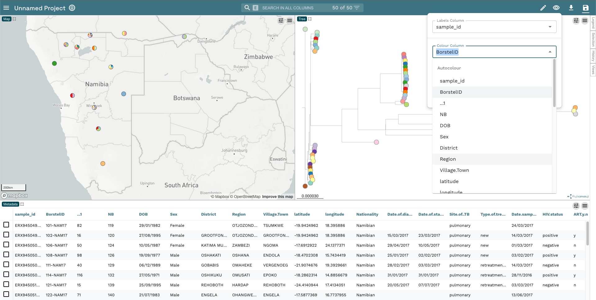
- This will change the colour of the tip nodes as well as the pie charts on the map - each region has its own colour as you’d expect:
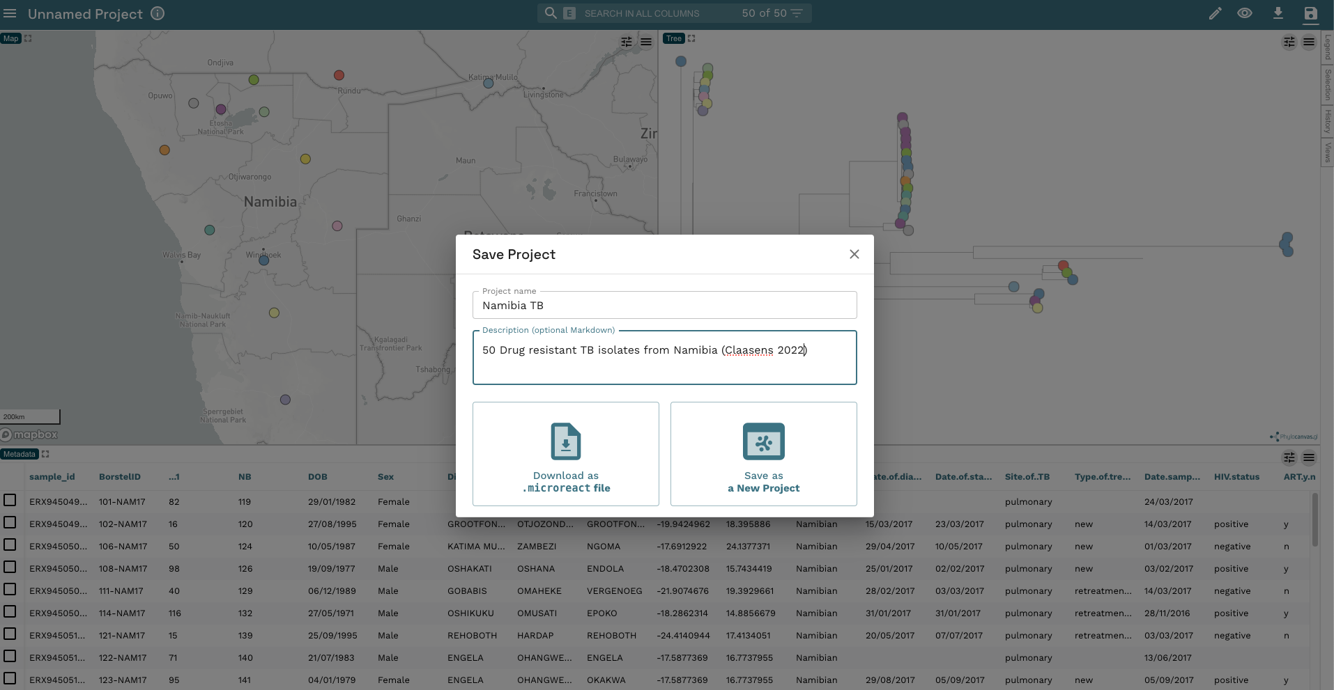
- At this point, before we proceed any further, let’s save the project to your accounts. Click on the Save button in the top-right corner, change the project name to Namibia TB and add some kind of description so you know what the dataset is. Then click Save as a New Project (another dialogue box will appear asking if you want to share your project; for now, close this box):
- Now, let’s make our phylogenetic tree a bit more informative. First, let’s add the tip labels to the display by clicking on the left-hand of the two buttons in the phylogeny window then the drop down arrow next to Nodes & Labels. Now click the slider next to Leaf Labels and the slider next to Align Leaf Labels. We’ll also make the text a little smaller by moving the slider to 12px:
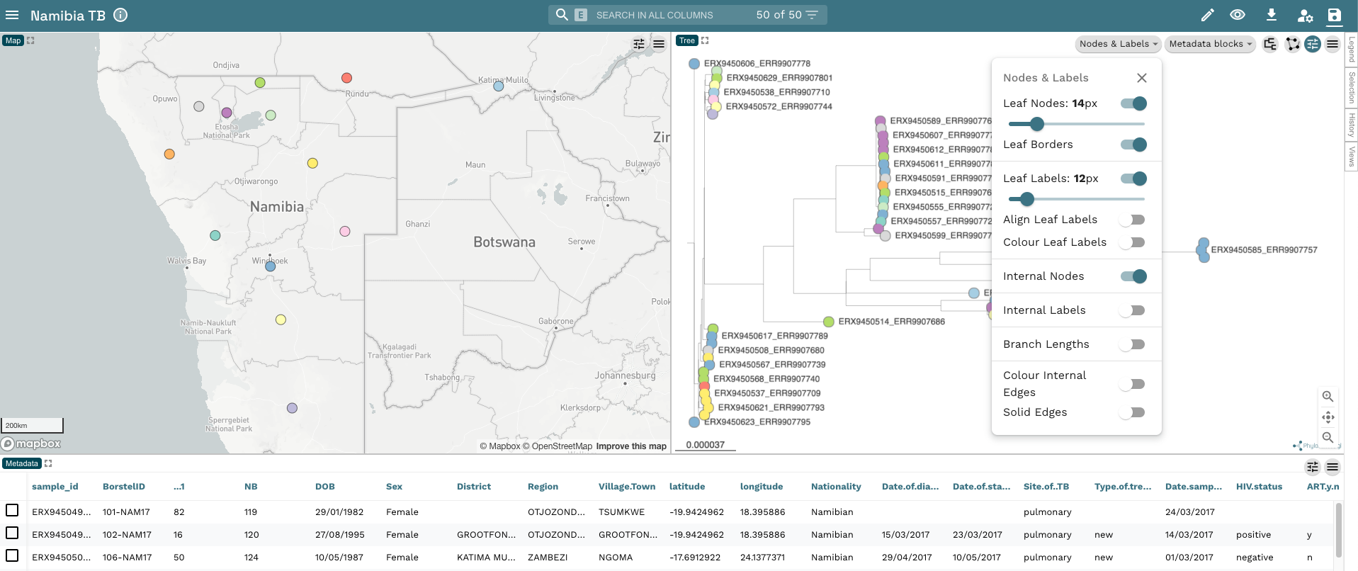
- The tip labels are still the European Nuclotide Accessions we used to download the FASTQ files. Let’s change the tip labels to the
BorstelIDwhich is what’s used in the paper. Click on the Eye icon again and change Labels Column toBorstelID:
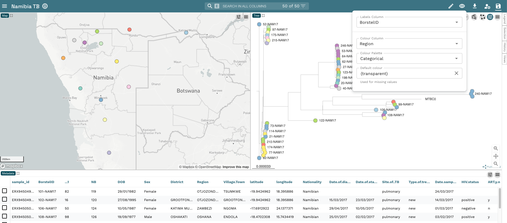
- From the rooted tree, we can see we have two distinct clades within the tree. These are the two major lineages we identified in our dataset (Lineage 2 and Lineage 4). To make this clearer, change the colour of the tip nodes to
main_lineageand click on Legend on the far right-hand side of the plot. Now we have a tree and map annotated with the two lineages in our dataset:
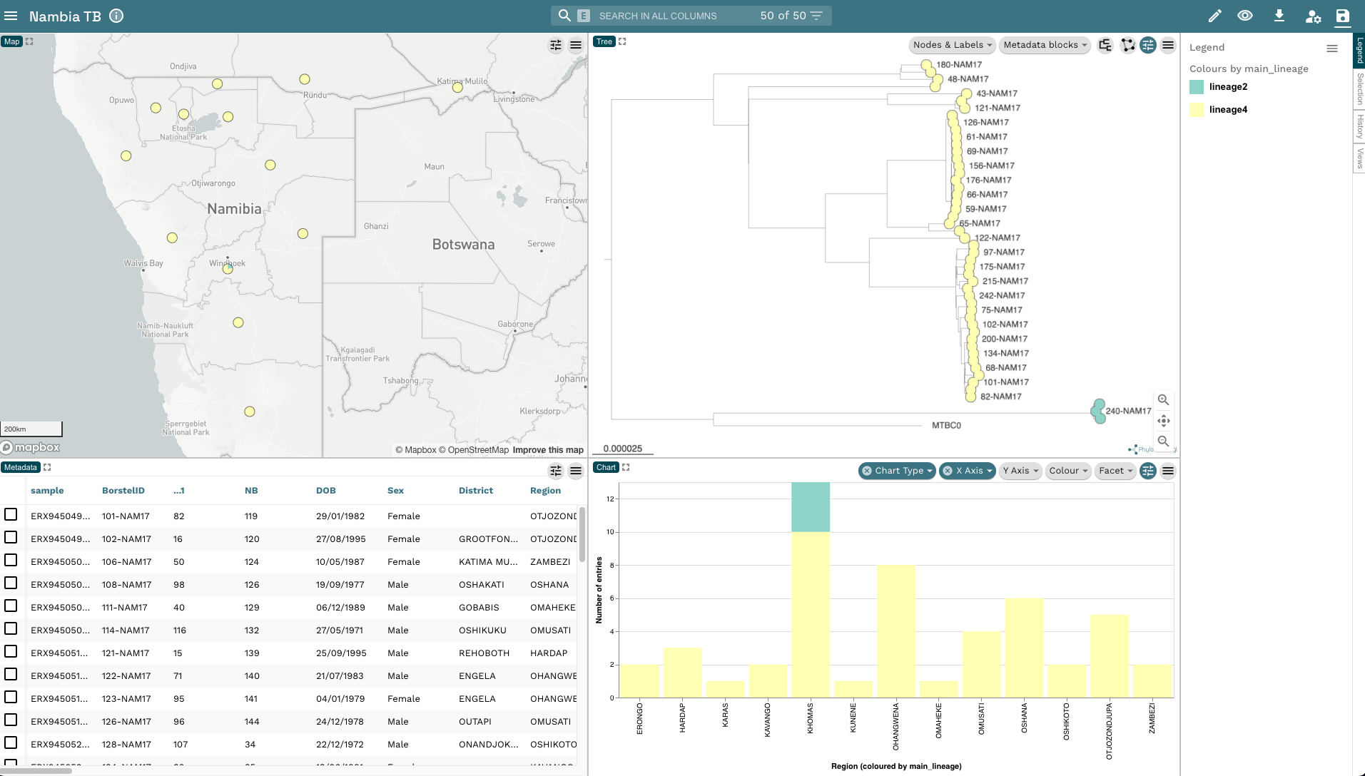
- The last thing we’re going to do is add a histogram to show the frequency of lineages across the different regions to our Microreact window. Click on the Pencil icon on the top-right corner and click Create New Chart then move your mouse into the right hand side of the metadata box at the bottom of the window and click when you see the blue box appear. A blank chart should appear. Click Chart Type and select Bar chart and change the X Axis Column to
Region. The plot should auto populate with the region on the X-axis and the Number of entries on the Y-axis. The bars are coloured according tomain_lineagewhich is what we’re currently using to colour our plots:
If you have information about which countries your samples come from, you can obtain latitude and longitude coordinates by using the Data-flo web application. Data-flo provides several convenience data transformation applications, one of which is called “Geocoder”.
- Go to data-flo.io
- On the top toolbar click on “Transformations”
- Search for “Geocoder”
- Click on “Run”
- Paste your country names in the “Inputs” box (you can copy these from your metadata table)
- Click “Run”
- Once it finishes, scroll all the way down and click on the file link “locations.csv” to download a file containing all the country coordinates
- You can then open your original metadata file and add these two columns to your metadata
Once you have this information, it will be possible to display your samples on a map using Microreact.
16.2 Summary
- Microreact is a free web app to visualise phylogenetic trees.
- It supports tree files in standard NEWICK format, as output by IQ-Tree.
- It also supports metadata for the samples, which can be used to configure the tree.
- Metadata such as latitude and longitude is also used to display the samples on a map.