14 Building phylogenetic trees
- Differentiate between common methods of tree inference and recognise why maximum likelihood is generally a preferable method of inference.
- Describe what are the key steps in creating a phylogenetic tree.
- Use
IQ-TREEfor phylogenetic tree inference from an alignment.
14.1 Phylogenetic tree inference
A phylogenetic tree is a graph (structure) representing evolutionary history and shared ancestry. It depicts the lines of evolutionary descent of different species, lineages or genes from a common ancestor. A phylogenetic tree is made of nodes and edges, with one edge connecting two nodes.
A node can represent an extant species, and extinct one, or a sampled pathogen: these are all cases of “terminal” nodes, nodes in the tree connected to only one edge, and usually associated with data, such as a genome sequence.
A tree also contains “internal” nodes: these usually represent most recent common ancestors (MRCAs) of groups of terminal nodes, and are typically not associated with observed data, although genome sequences and other features of these ancestors can be statistically inferred. An internal node is most often connected to 3 branches (two descendants and one ancestral), but a multifurcation node can have any number >2 of descendant branches.

14.1.1 Tree topology
A clade is the set of all terminal nodes descending from the same ancestor. Each branch and internal node in a tree is associated with a clade. If two trees have the same clades, we say that they have the same topology. If they have the same clades and the same branch lengths, the two tree are equivalent, that is, they represent the same evolutionary history.
14.1.2 Uses of phylogenetic trees
In many cases, the phylogenetic tree represents the end result of an analysis, for example if we are interested in the evolutionary history of a set of species.
However, in many cases a phylogenetic tree represents an intermediate step, and there are many ways in which phylogenetic trees can be used to help understand evolution and the spread of infectious disease.
In other cases, we may want to know more about genome evolution, for example about mutational pressures, but more frequently about selective pressures. Selection can affect genome evolution in many ways such as slowing down evolution of a portion of the genome in which changes are deleterious (“purifying selection”). Conversely, “positive selection” can favor changes at certain positions of the genome, effectively accelerating their evolution. Using genome data and phylogenetic trees, molecular evolution methods can infer different types of selection acting in different parts of the genome and different branches of a tree.
14.1.3 Newick format
We often need to represent trees in text format, for example to communicate them as input or output of phylogenetic inference software. The Newick format is the most common text format for phylogenetic trees.
The Newick format encloses each subtree (the part of a tree relating the terminal nodes part of the same clade) with parenthesis, and separates the two child nodes of the same internal node with a “,”. At the end of a Newick tree there is always a “;”.
For example, the Newick format of a rooted tree relating two samples “S1” and “S2”, with distances from the root respectively of 0.1 and 0.2, is
(S1:0.1,S2:0.2);
If we add a third sample “S3” as an outgroup, the tree might become
((S1:0.1,S2:0.2):0.3,S3:0.4);
14.1.4 Methods for inferring phylogenetic trees
A few different methods exist for inferring phylogenetic trees:
- Distance-based methods such as Neighbour-Joining and UPGMA
- Parsimony-based phylogenetics
- Maximum likelihood methods making use of nuclotide substitution models
Distance-based methods
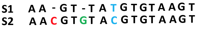
These are the simplest and fastest phylogenetic methods we can use and are often a useful way to have a quick look at our data before running more robust phylogenetic methods. Here, we infer evolutionary distances from the multiple sequence alignment. In the example below there is 1 subsitution out of 16 informative columns (we exclude columns with gaps or N’s) so the distance is approximately 1/16:
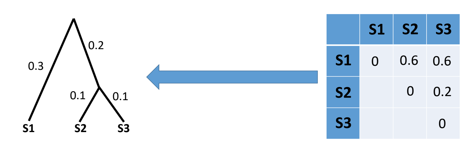
Typically, we have multiple sequences in an alignment so here we would generate a matrix of pairwise distances between all samples (distance matrix) and then use Neighbour-Joining or UPGMA to infer our phylogeny:
Parsimony methods
Maximum parsimony methods assume that the best phylogenetic tree requires the fewest number of mutations to explain the data (i.e. the simplest explanation is the most likely one). By reconstructing the ancestral sequences (at each node), maximum parsimony methods evaluate the number of mutations required by a tree then modify the tree a little bit at a time to improve it.
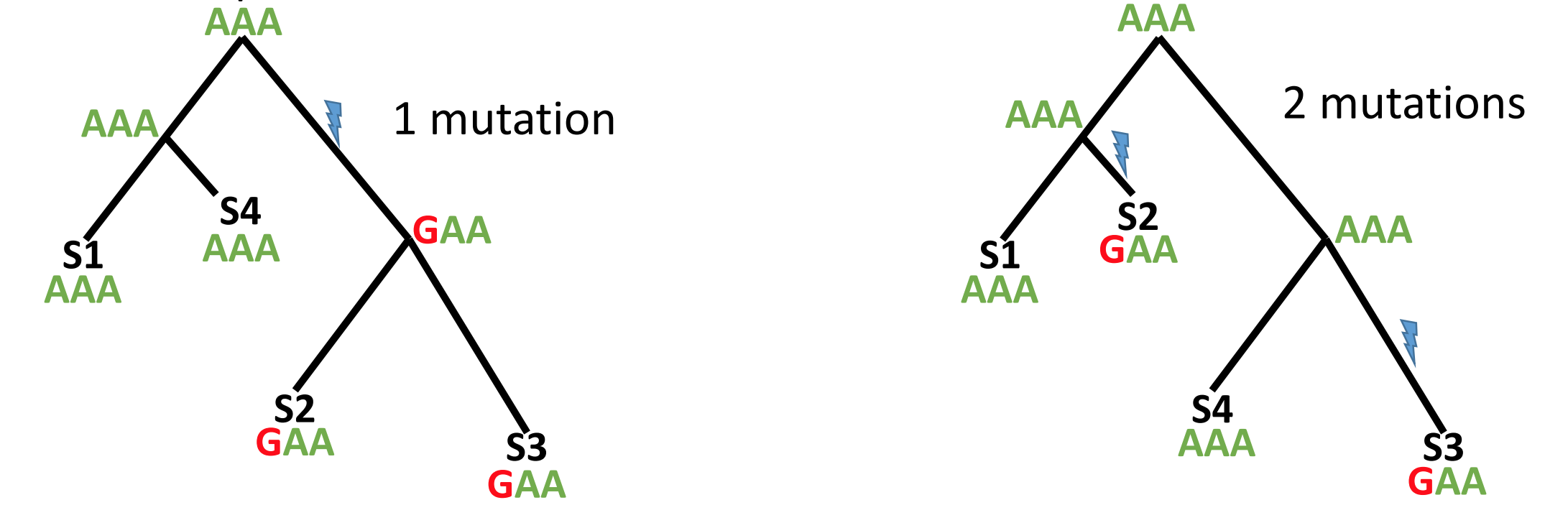
Maximum parsimony is an intuitive and simple method and is reasonably fast to run. However, because the most parsimonius tree is always the shortest tree, compared to the hypothetical “true” tree it will often underestimate the actual evolutionary change that may have occurred.
Maximum likelihood methods
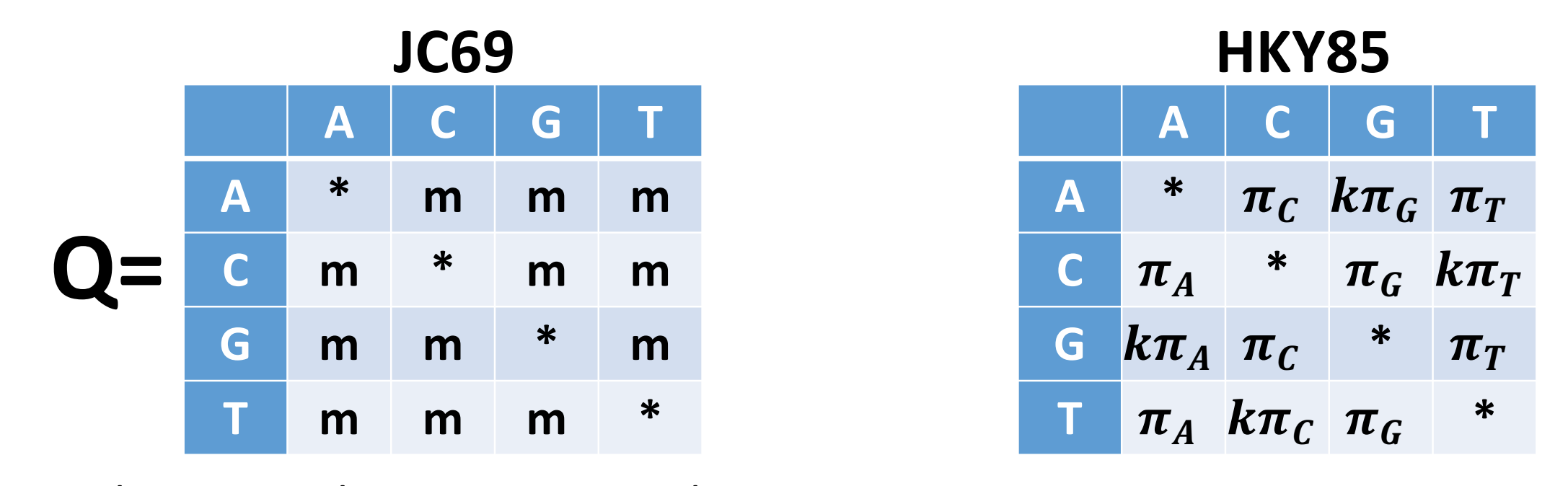
The most commonly encountered phylogenetic method when working with bacterial genome datasets is maximum likelihood. These methods use probabilistic models of genome evolution to evaluate trees and whilst similar to maximum parsimony, they allow statistical flexibility by permitting varying rates of evolution across different lineages and sites. This additional complexity means that maximum likelihood models are much slower than the previous two models discussed. Maximum likelihood methods make use of substitution models (models of DNA sequence evolution) that describe changes over evolutionary time. Two commonly used substitution models, Jukes-Cantor (JC69; assumes only one mutation rate) and Hasegawa, Kishino and Yano (HKY85; assumes different mutation rates - transitions have different rates) are depicted below:
It is also possible to incorporate additional assumptions about your data e.g. assuming that a proportion of the the alignment columns (the invariant or constant sites) cannot mutate or that there is rate variation between the different alignment columns (columns may evolve at different rates). The choice of which is the best model to use is often a tricky one; generally starting with one of the simpler models e.g. General time reversible (GTR) or HKY is the best way to proceed. Accounting for rate variation and invariant sites is an important aspect to consider so using models like HKY+G4+I (G4 = four types of rate variation allowed; I = invariant sites don’t mutate) should also be considered.
There are a number of different tools for phylogenetic inference via maximum-likelihood and some of the most popular tools used for phylogenetic inference are FastTree, IQ-TREE and RAxML-NG. For this lesson, we’re going to use IQ-TREE as it is fast and has a large number of substitution models to consider. It also has a model finder option which tells IQ-TREE to pick the best fitting model for your dataset, thus removing the decision of which model to pick entirely.
14.1.5 Tree uncertainty - bootstrap
All the methods for phylogenetic inference that we discussed so far aim at estimating a single realistic tree, but they don’t automatically tell us how confident we should be in the tree, or in individual branches of the tree.
One common way to address this limitation is using the phylogenetic bootstrap approach (Felsenstein, 1985). This consists of first sampling a large number (say, 1000) of bootstrap alignments. Each of these alignments has the same size as the original alignment, and is obtained by sampling with replacement the columns of the original alignment; in each bootstrap alignment some of the columns of the original alignment will usually be absent, and some other columns would be represented multiple times. We then infer a bootstrap tree from each bootstrap alignment. Because the bootstrap alignments differ from each other and from the original alignment, the bootstrap trees might different between each other and from the original tree. The bootstrap support of a branch in the original tree is then defined as the proportion of times in which this branch is present in the bootstrap trees.
14.2 Multiple sequence alignments
Phylogenetic methods require sequence alignments. These can range from alignments of a single gene from different species to whole genome alignments where a sample’s sequence reads are mapped to a reference genome. Alignments attempt to place nucleotides from the same ancestral nucleotide in the same column. One of the most commonly used alignment formats in phylogenetics is FASTA:
>Sample_1
AA-GT-T
>Sample_2
AACGTGT
N and - characters represent missing data and are interpreted by phylogenetic methods as such.
The two most commonly used muliple sequence alignments in bacterial genomics are reference-based whole genome alignments and core genome alignments generated by comparing genes between different isolates and identifying the genes found in all or nearly all isolates (the core genome). As a broad rule of thumb, if your species is not genetically diverse and doesn’t recombine (TB, Brucella) then picking a suitable good-quality reference and generating a whole genome alignment is appropriate. However, when you have a lot of diversity or multiple divergent lineages (E. coli) then a single reference may not represent all the diversity in your dataset. Here it would be more typical to create de novo assemblies, annotate them and then use a tool like roary or panaroo to infer the pan-genome and create a core genome alignment. The same phylogenetic methods are then applied to either type of multiple sequence alignment.
14.3 Building a phylogenetic tree
Following that very brief introduction to phylogenetics, we can start building our first phylogenetic tree using the masked alignment file we created in the previous section.
We start our analysis by activating our software environment, to make all the necessary tools available:
mamba activate iqtree14.3.1 Extracting variable sites with SNP-sites
Although you could use the alignment generated by bactmap directly as input to IQ-TREE, this would be quite computationally intensive, because the whole genome alignments tend to be quite large. Instead, what we can do is extract the variable sites from the alignment, such that we reduce our FASTA file to only include those positions that are variable across samples i.e. the positions that are phylogenetically informative.
Here is a small example illustrating what we are doing. For example, take the following three sequences, where we see 3 variable sites (indicated with an arrow):
seq1  C G T A G C T G G T
seq2  C T T A G C A G G T
seq3  C T T A G C A G A T
        ↑         ↑   ↑
For the purposes of phylogenetic tree construction, we only use the variable sites to look at the relationship between our sequences, so we can simplify our alignment by extract only the variable sites:
seq1  G T G
seq2  T A G
seq3  T A A
This example is very small, but when you have megabase-sized genomes, this can make a big difference. To extract variable sites from an alignment we can use the snp-sites software:
# create output directory
mkdir results/snp-sites

# run SNP-sites
snp-sites results/bactmap/masked_alignment/aligned_pseudogenomes_masked.fas -o results/snp-sites/aligned_pseudogenomes_masked_snps.fas
This command simply takes as input the alignment FASTA file and produces a new file with only the variable sites - which we save (-o) to an output file. This is the file we will use as input to constructing our tree. However, before we move on to that step, we need another piece of information: the number of constant sites in the initial alignment (sites that didn’t vary in our alignment). Phylogenetically, it makes a difference if we have 3 mutations in 10 sites (30% variable sites, as in our small example above) or 3 mutations in 1000 sites (0.3% mutations). The IQ-TREE software we will use for tree inference can accept as input 4 numbers, counting the number of A, C, G and T that were constant in the alignment. For our small example above these would be, respectively: 1, 2, 2, 2.
Fortunately, the snp-sites command can also produce these numbers for us (you can check this in the help page by running snp-sites -h). This is how you would do this:
# count invariant sites
snp-sites -C results/bactmap/masked_alignment/aligned_pseudogenomes_masked.fas > results/snp-sites/constant_sites.txt
The key difference is that we use the -C option, which produces these numbers. We redirect (>) the output to a file. We can see what these numbers are by printing the content of the file:
cat results/snp-sites/constant_sites.txt692240,1310839,1306835,691662As we said earlier, these numbers represent the number of A, C, G, T that were constant in our original alignment. We will use these numbers in the tree inference step detailed next.
14.3.2 Tree inference with IQ-TREE
There are different methods for inferring phylogenetic trees from sequence alignments. Regardless of the method used, the objective is to construct a tree that represents the evolutionary relationships between different species or genetic sequences. Here, we will use the IQ-TREE software, which implements maximum likelihood methods of tree inference. IQ-TREE offers various sequence evolution models, allowing researchers to match their analyses to different types of data and research questions. Conveniently, this software can identify the most fitting substituion model for a dataset (using a tool called ModelFinder), while considering the complexity of each model.
We run IQ-TREE on the output from snp-sites, i.e. using the variable sites extracted from the core genome alignment:
# create output directory
mkdir results/iqtree

# run iqtree2
iqtree \
  -s results/snp-sites/aligned_pseudogenomes_masked_snps.fas \
  -fconst 692240,1310839,1306835,691662 \
  --prefix results/iqtree/Nam_TB \
  -nt AUTO \
  -ntmax 8 \
  -mem 8G \
  -m GTR+F+I \
  -bb 1000
The options used are:
-s- the input alignment file, in our case using only the variable sites extracted withsnp-sites.--prefix- the name of the output files. This will be used to name all the files with a “prefix”. In this case we are using the “Nam_TB” prefix, which refers to the data we’re using.-fconst- these are the counts of invariant sites we estimated in the previous step withsnp-sites(see previous section).-nt AUTO- automatically detect how many CPUs are available on the computer for parallel processing (quicker to run).-ntmax 8- set the maximum number of CPUs to use-mem 8G- set the maximum amount of RAM to use-m- specifies the DNA substitution model we’d like to use. We give more details about this option below.-bb 1000- run 1000 fast bootstraps. See the section on bootstrapping above.
When not specifying the -m option, IQ-TREE employs ModelFinder to pinpoint the substitution model that best maximizes the data’s likelihood, as previously mentioned. Nevertheless, this can be time-consuming (as IQ-TREE needs to fit trees numerous times). An alternative approach is utilizing a versatile model, like the one chosen here, “GTR+F+I,” which is a generalized time reversible (GTR) substitution model. This model requires an estimate of the base frequencies within the sample population, determined in this instance by tallying the base frequencies from the alignment (indicated by “+F” in the model name). Lastly, the model accommodates variations in rates across sites, including a portion of invariant sites (noted by “+I” in the model name).
We can look at the output folder:
ls results/iqtreeNam_TB.bionj Nam_TB.log Nam_TB.mldist
Nam_TB.ckp.gz Nam_TB.iqtree Nam_TB.treefileThere are several files with the following extensions:
.iqtree- a text file containing a report of the IQ-Tree run, including a representation of the tree in text format..treefile- the estimated tree in NEWICK format. We can use this file with other programs, such as FigTree, to visualise our tree..log- the log file containing the messages that were also printed on the screen..bionj- the initial tree estimated by neighbour joining (NEWICK format)..mldist- the maximum likelihood distances between every pair of sequences..ckp.gz- this is a “checkpoint” file, which IQ-Tree uses to resume a run in case it was interrupted (e.g. if you are estimating very large trees and your job fails half-way through).
The main files of interest are the report file (.iqtree) and the tree file (.treefile) in standard Newick format.
14.3.3 Rooting a phylogenetic tree
Rooting a phylogenetic tree is essential for making sense of evolutionary relationships and for providing a temporal context to the diversification of species. It transforms an unrooted tree, which simply shows relationships without direction, into a meaningful representation of evolutionary history. The most common way to accurately root a phylogenetic tree is to include an outgroup that is known to be more distantly related to the taxa included as part of the analysis. In our example we mapped our TB sequences to the MTBC0 reference, which is an outgroup to all members of the MTBC, so we’ll use this to root our tree before visualizing it. There are a few different tools that could be used to root a phylogenetic tree but we’ve provided a python script, root_tree.py to do this. You can run the script using the following command (we’re going to root the tree we’ve provided in the preprocessed directory so you don’t need to edit the command):
python scripts/root_tree.py -i preprocessed/iqtree/Nam_TB.treefile -g MTBC0 -o results/iqtree/Nam_TB_rooted.treefileThe options we used are:
-i- the TB phylogenetic tree we inferred withIQ-TREE.-g- the name of the outgroup to root the tree with (in this case MTBC0).-o- the rooted phylogenetic tree.
This will create a NEWICK file called Nam_TB_rooted.treefile in your results directory.
14.4 Summary
- Tree inference methods include neighbor-joining, maximum parsimony and maximum likelihood. The first two are simpler and computationally faster, but do not accurately capture relevant features of sequence evolution.
- Maximum likelihood methods are recommended, as they incorporate relevant parameters such as different substitution rates, invariant sites and variable mutation rates across the sequence.
- Phylogenetic tree inference requires a multiple sequence alignment as input, regardless of which method of inference is used.
- To reduce the computational burden of the analysis when using whole-genome alignments, we can extract variable sites from our alignment using the
snp-sitessoftware. - IQ-Tree is a popular software for maximum likelihood tree inference and can take as input the variable sites from the previous step.