# Load libraries
library(Seurat) # single-cell and spatial analysis toolkit
library(sparseMatrixStats)
library(paletteer) # colour palettes
library(ggplot2) # plotting
library(dplyr) # data manipulation
library(patchwork) # combining plots

# Load the Seurat object from the previous chapter
visium <- readRDS("precomputed/mouse_brain_clustering.rds")9 Cluster Marker Genes
TipLearning Objectives
- Explain why marker gene analysis after clustering is exploratory and should be validated with external data.
- Identify marker genes for each cluster and interpret the main columns in the output table.
- Filter marker genes to find significant, high-effect markers and visualiase their spatial expression patterns.
9.1 Setup
We continue working with the sagittal mouse brain dataset from previous chapters.
NoteClick to expand
Start by loading the required libraries and the Seurat object.
As a reminder, this object was created by:
- Importing the raw data using
Load10X_Spatial(), followed by QC and filtering to remove low-quality spots. - Data normalisation using
SCTransform(), which models technical variation and applies variance stabilisation. Stored in the “SCT” assay. - Applying dimensionality reduction using PCA, UMAP and t-SNE.
- Clustering the data using graph-based clustering. The clusters we use in this chapter were generated using the Leiden algorithm at a resolution of 0.8 and were set the the default cell identities (
Idents(visium)).
9.2 Overview
Following from our clustering, a natural next step is to understand what each cluster represents biologically. To do this, we identify marker genes, i.e. genes that are differentially expressed between the clusters.
It is worth noting that this procedure is statistically flawed and can lead to misleading conclusions. The reason being that our clusters were defined based on gene expression patterns, so we are not testing independent hypotheses. In other words, we should expect to find significant markers for each cluster, as the clusters themselves were defined based on gene expression pattern differences. This is true, even if the clusters are not biologically meaningful. For that reason, this analysis should be considered exploratory and hypothesis-generating, rather than a rigorous statistical test. The marker genes we identify can be used to assign biological identity to the clusters, but this should be done with caution and ideally validated using external data or experiments.
There are several statistical tests used for marker gene identification. For the reason mentioned above, we shouldn’t worry too much about being “statistically rigorous” here, so simple approaches are often sufficient. In fact, one of the most commonly used tests is the Wilcoxon rank-sum test, which is a generic non-parametric test that compares the ranking of expression of each gene in one cluster against the others. This test is robust to outliers and does not assume a specific distribution.
Tests specifically designed for single-cell data (e.g. MAST) can better account for variable detection rates across cells, but can be computationally more intensive. For spatial transcriptomics data with fewer cells and often lower sparsity than single-cell data, the Wilcoxon test typically performs well and is sufficiently fast.
9.3 Find Marker Genes
Seurat provides the function FindAllMarkers() to perform differential expression analysis between a target cluster and all other clusters.
Some critical parameters of this function to consider are:
only.pos: IfTRUE, only returns markers that are more highly expressed in the cluster of interest.min.pct: The minimum percentage of cells/spots in the cluster where the gene is detected (default 0.1). Raising this threshold prevents genes expressed in just a few spots from dominating the marker list.logfc.threshold: the minimum log-fold change in expression for a gene to be considered for testing.
Both min.pct and logfc.threshold are should be set to relatively permissive values, as their main purpose is to reduce the computational burden of testing genes that are unlikely to be markers. These parameters trade off sensitivity (finding all true markers) against specificity (avoiding false positives). Stricter thresholds produce fewer, higher-confidence markers, while relaxed thresholds result in more markers but may include noisy results.
Let’s apply FindAllMarkers() to our Visium data and explore the results.
# Identify marker genes for each cluster
# Expressed in at least 5% of spots in the cluster, with a log-fold change of at least 0.25
markers <- FindAllMarkers(
  visium,
  only.pos = TRUE,
  min.pct = 0.25,
  logfc.threshold = 0.25
)

# The result is a standard data.frame
head(markers)
p_val avg_log2FC pct.1 pct.2 p_val_adj cluster gene
Adora2a 1.697275e-314 3.797143 0.958 0.197 3.061035e-310 1 Adora2a
Drd2 1.455810e-301 3.791027 0.915 0.162 2.625554e-297 1 Drd2
Rgs9 1.194384e-271 3.427709 0.980 0.374 2.154071e-267 1 Rgs9
Syndig1l 5.526844e-271 3.424814 0.948 0.258 9.967664e-267 1 Syndig1l
Gpr6 2.469811e-270 3.854899 0.807 0.109 4.454305e-266 1 Gpr6
Pde10a 9.983153e-268 3.383378 1.000 0.634 1.800462e-263 1 Pde10aThe result of this function is a standard R data frame with the following columns:
pvalis the p-value from the statistical testavg_log2FCis the average log2 fold change of the gene in the cluster compared to otherspct.1is the percentage of spots in the cluster where the gene is detectedpct.2is the percentage of spots in the other clusters where the gene is detectedp_val_adjis the p-value adjusted for multiple testingclusteris the cluster for which the gene is a markergeneis the name of the gene
9.4 Filtering Results
We can manipulate the output table using dplyr (part of tidyverse), to combine several criteria to find the most potentially interesting markers.
For example, in the code below, we filter for significant markers (adjusted p-value < 0.05). Then, for each cluster, we take the top 5 genes with the highest log-fold change.
# View top 5 markers for each cluster
top5 <- markers |>
  # filter for significant markers (adjusted p-value < 0.05)
  filter(p_val_adj < 0.05) |>
  # then for each cluster
  group_by(cluster) |>
  # take the top 5 genes with the highest log-fold change
  slice_max(avg_log2FC, n = 5) |>
  # sort them by cluster and descending log-fold change
  arrange(cluster, desc(avg_log2FC)) |>
  # reset grouping
  ungroup()

# Genes in cluster 1
top5 |>
  filter(cluster == 1) |>
  pull(gene)
[1] "Ido1" "Cd4" "Serpina9" "Gpr6" "Adora2a" We can visualise the expression of these marker genes across the tissue using SpatialFeaturePlot(), which shows the spatial distribution of gene expression.
# Visualise the 5 top markers for cluster 1
feature_plot <- SpatialFeaturePlot(
  visium,
  features = top5 |> filter(cluster == 1) |> pull(gene),
  ncol = 2
)

# Visualise the spatial location of cluster 1
cluster_plot <- SpatialDimPlot(
  visium,
  cells.highlight = WhichCells(visium, idents = "1")
) +
  ggtitle("Cluster 1 Spatial Location")

# Plot side by side
feature_plot + cluster_plot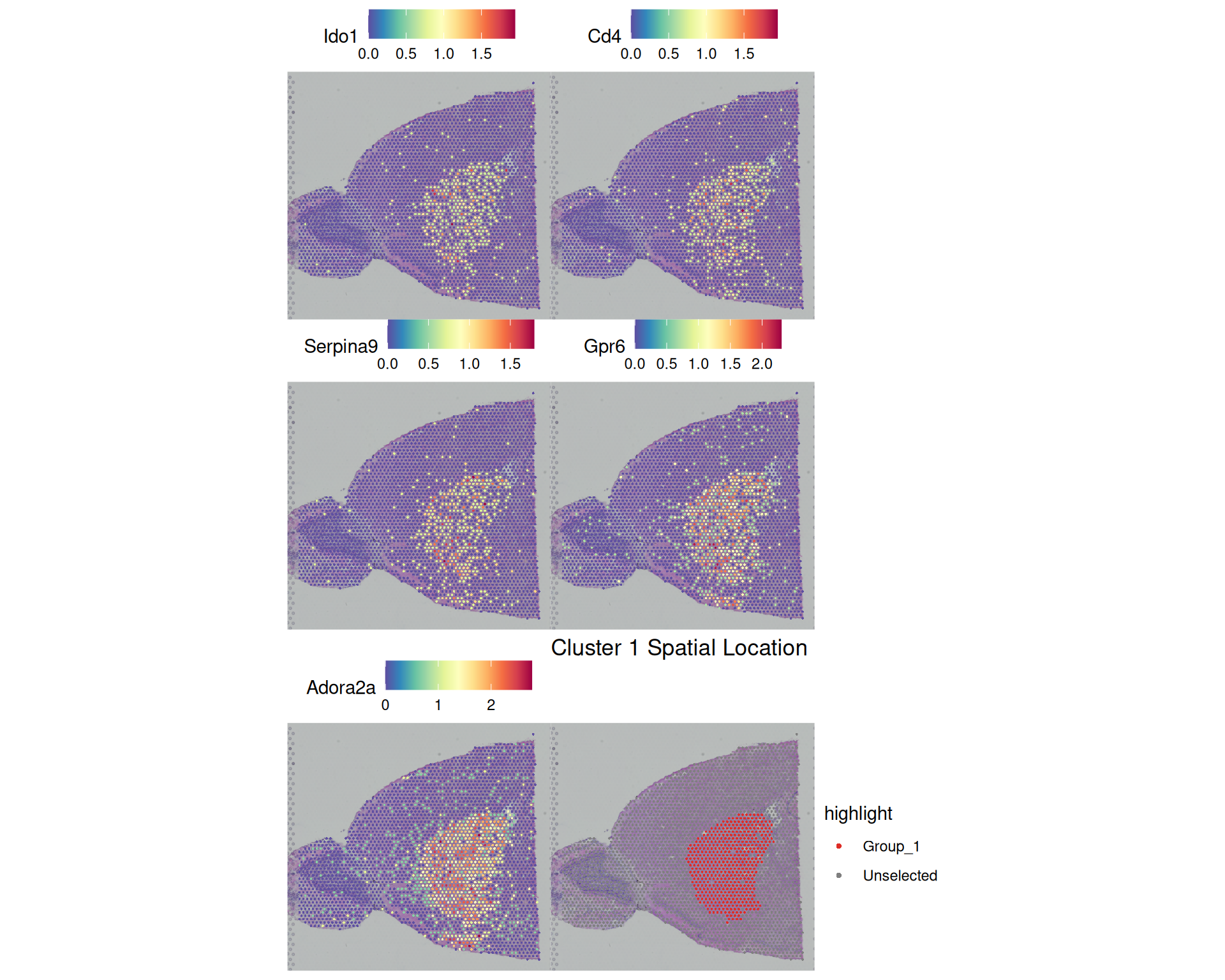
Another way you can filter this table is based on the pct.1 and pct.2 columns, which represent the fraction of spots where the gene was detected in the target cluster and in other clusters, respectively. For example, below we set the very strict criteria that the gene has to be detected in all spots of the target spot, and in no more than 50% of the rest of the spots:
# Filter on percent detected
top_by_pct <- markers |>
  filter(p_val_adj < 0.05 & pct.1 == 1 & pct.2 < 0.5)

# Count how many genes we have per cluster
top_by_pct |>
  count(cluster)
cluster n
1 8 3
2 10 1
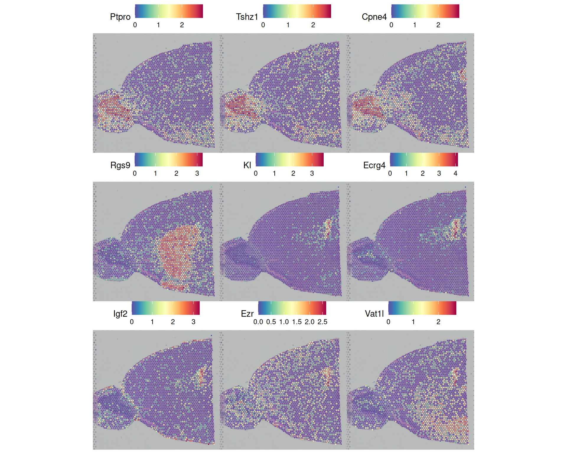
3 11 5This only returns 9 in only a few of the clusters. We could visualise these to see how specifically localised they are in our tissue:
# Visualise the top markers based on pct filtering
SpatialFeaturePlot(
  visium,
  features = top_by_pct$gene,
  ncol = 3
)
We could follow-up by comparing these markers to literature or reference datasets, to start assigning biological meaning identity to these clusters. You could also perform gene ontology analysis and pathway analysis on the marker genes for each cluster, to identify enriched biological processes or pathways. In this case, you may want to use more relaxed filtering criteria to get a larger list of genes for the analysis, for example: p_val_adj < 0.05 & avg_log2FC > log2(3) to get significant genes with at least a 3x fold change.
9.5 Summary
TipKey Points
- Marker gene analysis helps label clusters, but it is exploratory because the clusters were already defined from expression data.
- Use the results to generate hypotheses about cluster identity.
- Validate suggested identities with external reference data or experiments.
FindAllMarkers()compares each cluster against all others and returns a data frame with the results.- The Wilcoxon rank-sum test is a common statistical test choice for spatial transcriptomics data.
only.pos = TRUEkeeps only genes upregulated in the target cluster.min.pctandlogfc.thresholdhelp exclude genes unlikely to show differences for computational efficiency.
- Marker genes for each cluster can be identified by filtering on p-values, log-fold changes, and/or the percentage of spots expressing the gene.
- Filtering criteria should be chosen based on the specific goal, for example: stricter thresholds for identifying highly specific markers; more permissive thresholds for performing a follow-up gene ontology analysis.
- Marker genes can be visualised using spatial plots of gene expression.