# Load libraries
library(Seurat) # single-cell and spatial analysis toolkit
library(sparseMatrixStats)
library(paletteer) # colour palettes
library(ggplot2) # plotting
library(dplyr) # data manipulation
library(patchwork) # combining plots

# Load the Seurat object from the previous chapter
visium <- readRDS("precomputed/mouse_brain_svgs.rds")11 Spatial Clustering
TipLearning Objectives
- Use BANKSY to augment gene expression data with spatial features and perform spatially-aware clustering.
- Interpret BANKSY clusters and explain how they differ from non-spatial clustering results.
- Identify relationships between BANKSY clusters, spatially variable genes, and cell type identities.
- Adjust BANKSY parameters (
lambdaandk_geom) to control the balance between spatial and transcriptional similarity.
11.1 Setup
We continue working with the sagittal mouse brain dataset from previous chapters.
NoteClick to expand
Start by loading the required libraries and the Seurat object.
As a reminder, this object was created by:
- Importing the raw data using
Load10X_Spatial(), followed by QC and filtering to remove low-quality spots. - Data normalisation using
SCTransform(), which models technical variation and applies variance stabilisation. Stored in the “SCT” assay. - Applying dimensionality reduction using PCA, UMAP and t-SNE.
- Clustering the data using graph-based clustering. The clusters we use in this chapter were generated using the Leiden algorithm at a resolution of 0.8 and were set the the default cell identities (
Idents(visium)). - Identifying spatially variable features using Moran’s I and markvariogram methods.
11.2 Overview
In our previous clustering chapter, we grouped spots based solely on transcriptional similarity, without considering spatial organisation.
Tissue architecture describes the spatial organisation and arrangement of cell types within tissue. To capture this, we need clustering methods that incorporate spatial information alongside gene expression.
BANKSY is a spatially aware clustering method that combines gene expression with spatial context. Unlike standard graph-based clustering, BANKSY first enriches the gene expression matrix by adding spatial features, then clusters using this augmented representation.
For each gene, BANKSY calculates two spatial features:
- Mean neighbourhood expression: The average expression of a gene across neighbouring spots, weighted so nearby spots contribute more strongly than distant ones.
- Azimuthal Gabor filter (AGF): Inspired by image processing, this captures directional changes in expression around each spot by measuring how expression differs across the neighbourhood. It highlights spots that deviate from their surrounding tissue environment.
BANKSY combines these spatial features with the original gene expression values before clustering. The result is that BANKSY identifies tissue domains defined by both gene expression and spatial patterns.
11.3 Running BANKSY
BANKSY is built on Bioconductor’s SpatialExperiment class, but the SeuratWrappers package provides a convenient interface to run BANKSY directly on Seurat objects. Load these packages:
# Load necessary libraries
library(SeuratWrappers)
library(Banksy)
The RunBanksy() function accepts two key parameters that control clustering:
lambda: Controls the balance between spatial and transcriptional information.lambda = 0uses only transcriptional information (equivalent to standard graph-based clustering).lambda = 1uses only spatial information from the neighbourhood.- Values in between give a weighted balance between spatial domains and cell identities.
k_geom: Controls the number of spatial neighbours used to calculate mean neighbourhood expression and the azimuthal Gabor filter. Larger values include more distant neighbours. Note that the samek_geomvalue corresponds to very different physical areas depending on the spatial resolution of the technology (discussed below).
By default, RunBanksy() does not calculate AGF features (as it is computationally intensive), but you can enable this with use_agf = TRUE. We use all genes for the analysis to keep it independent of previous variable feature selection.
# Run BANKSY on the Seurat object
visium <- RunBanksy(
  visium,
  assay = "SCT",
  lambda = 0.2,
  k_geom = 18,
  use_agf = TRUE,
  features = "all"
)
# Confirm that the BANKSY assay has been added to the Seurat object
Assays(visium)[1] "Spatial" "SCT" "Scran" "BANKSY" # Check the layers in the BANKSY assay
Layers(visium[["BANKSY"]])[1] "data" "scale.data"RunBanksy() creates a new assay (by default named “BANKSY”) containing the augmented gene expression matrix with a scale.data layer ready for downstream analysis. This matrix has three times as many features as the original assay: the original gene expression plus mean neighbourhood expression and AGF features for each gene.
# Compare the dimensions of the SCT and BANKSY assays
nrow(visium[["SCT"]])
[1] 18035nrow(visium[["BANKSY"]])[1] 5410511.3.1 Clustering
With the augmented BANKSY gene expression, we proceed to cluster the data using standard steps:
- Run PCA on the BANKSY assay to reduce dimensionality.
- Find nearest neighbours based on the PCA reduction.
- Cluster the data using graph-based clustering (Leiden or Louvain).
We use 50 principal components and a resolution of 0.8 for the Leiden algorithm, matching our previous analysis. We store the new cluster identities in a column called “banksy_cluster” to distinguish them from the earlier non-spatial clusters.
# Cluster based on BANKSY assay
visium <- visium |>
  RunPCA(
    assay = "BANKSY",
    reduction.name = "pca_banksy",
    reduction.key = "pcabanksy_",
    features = rownames(visium[["BANKSY"]]),
    npcs = 50
  ) |>
  FindNeighbors(reduction = "pca_banksy", dims = 1:50) |>
  FindClusters(cluster.name = "banksy_cluster", resolution = 0.8)
Modularity Optimizer version 1.3.0 by Ludo Waltman and Nees Jan van Eck
Number of nodes: 2780
Number of edges: 71114
Running Louvain algorithm...
Maximum modularity in 10 random starts: 0.8782
Number of communities: 18
Elapsed time: 0 seconds# Run UMAP on the BANKSY PCA reduction
visium <- RunUMAP(
visium,
reduction = "pca_banksy",
dims = 1:50,
reduction.name = "umap_banksy"
)11.3.2 Visualisation
We next visualise the BANKSY clusters on UMAP and spatial plots to see how they relate to tissue organisation. For comparison, we also display the earlier non-spatial clusters.
Show code for BANKSY cluster visualisation
# UMAP plot
banksy_umap <- DimPlot(
  visium,
  reduction = "umap_banksy",
  group.by = "banksy_cluster",
  label = TRUE
) +
  ggtitle("BANKSY Clusters: lambda = 0.2, k_geom = 18") +
  theme_void()

# Spatial plot
banksky_spatial <- SpatialDimPlot(
  visium,
  group.by = "banksy_cluster",
  label = TRUE,
  label.size = 4,
  image.alpha = 0.5
) +
  theme(legend.position = "none")

# SCT assay UMAP and spatial plots for comparison
sct_umap <- DimPlot(
  visium,
  reduction = "umap",
  group.by = "Leiden_08",
  label = TRUE
) +
  ggtitle("SCT Clusters") +
  theme_void()

sct_spatial <- SpatialDimPlot(
  visium,
  group.by = "Leiden_08",
  label = TRUE,
  label.size = 4,
  image.alpha = 0.5
) +
  theme(legend.position = "none")

# Highlight a particular cluster of interest
sct_c5_umap <- DimPlot(
  visium,
  reduction = "umap",
  cells.highlight = WhichCells(visium, expression = Leiden_08 == "5"),
  label = TRUE
) +
  ggtitle("SCT Cluster 5") +
  theme_void()

sct_c5_spatial <- SpatialPlot(
  visium,
  cells.highlight = WhichCells(visium, expression = Leiden_08 == "5"),
  image.alpha = 0.5
) +
  ggtitle("SCT cluster 5") +
  theme(legend.position = "none")

# Plot side by side
(banksy_umap + banksky_spatial) /
  (sct_umap + sct_spatial) /
  (sct_c5_umap + sct_c5_spatial)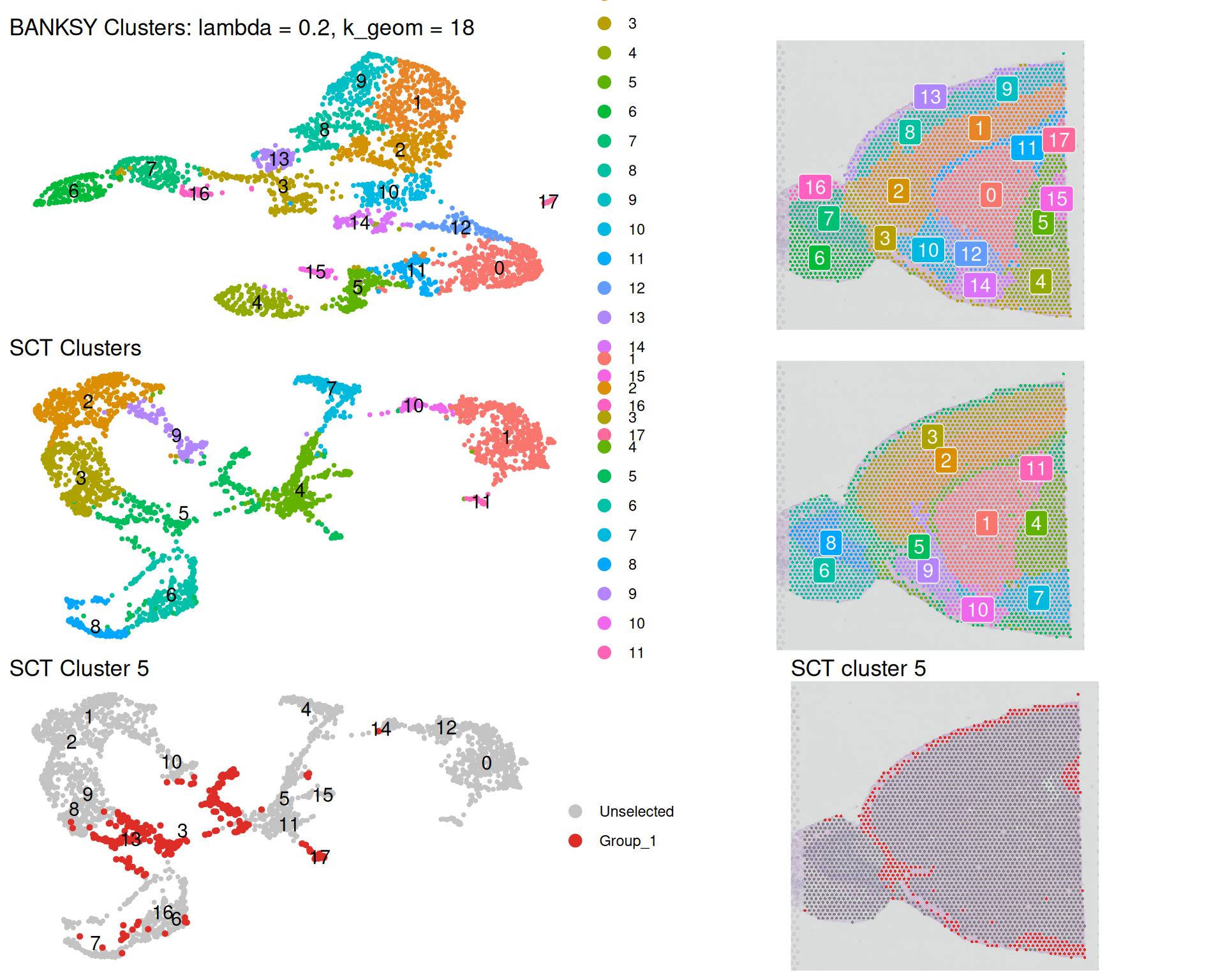
The BANKSY UMAP differs from the SCT UMAP because BANKSY incorporates spatial information. Notice the reduced mixing in both plots, indicating tighter spatial coherence. For example, non-spatial cluster 5 is split across several separate regions of the tissue. BANKSY fragments this scattered cluster into more spatially unified domains.
This shows how BANKSY emphasises tissue architecture. Even with a relatively modest lambda value of 0.2, spatial structure emerges clearly.
We also see what might be some artefacts in the BANKSY clusters. For example, spots from the olfactory bulb (on the left) are placed in cluster 2, which might not be biologically correct. As always, knowledge of the biology would help interpret and judge the validity of these results.
It is important to understand that BANKSY clusters are not “better” than non-spatial clusters, rather they answer different biological questions. Non-spatial clustering identifies cell identities: groups of cells with similar transcriptional profiles, regardless of location. The same cell type may appear in different tissue regions. BANKSY identifies tissue domains: spatial regions defined by both transcriptional profiles and spatial context. A tissue domain may contain multiple cell types but represents a coherent spatial unit.
ImportantChoosing
lambda appropriately
We copy guidance directly from the BANKSY documentation, as it applies to our dataset:
An important note about choosing the
lambdaparameter for the older Visium v1 / v2 55um > datasets or the original ST 100um technology:For most modern high resolution technologies like Xenium, Visium HD, StereoSeq, MERFISH, STARmap PLUS, SeqFISH+, SlideSeq v2, and CosMx (and others), we recommend the usual defults for
lambda: For cell typing, uselambda = 0.2(as shown below, or in this > vignette) and for domain > segmentation, uselambda = 0.8. These technologies are either imaging based, having true single-cell resolution (e.g., MERFISH), or are sequencing based, having barcoded spots on the scale of single-cells (e.g., Visium > HD). We find that the usual defaults work well at this measurement resolution.However, for the older Visium v1/v2 or ST technologies, with their much lower resolution spots (55um and 100um diameter, respectively), we find that
lambda = 0.2seems to work best for domain segmentation. This could be because each spot already measures the average transcriptome of several cells in a neighbourhood. It seems thatlambda = 0.2shares enough information between these neighbourhoods to lead to good domain segmentation performance. For example, in the human DLPFC > vignette, we uselambda = 0.2on a Visium v1/v2 dataset. Also note that in these lower resolution technologies, each spot can have multiple cells of different types, and as such cell-typing is not defined for them.
ImportantChoosing
k_geom appropriately
The k_geom parameter controls the number of spatial neighbours used to calculate neighbourhood metrics. It is helpful to think of k_geom in terms of the physical spatial radius it represents rather than just the number of neighbours.
The same k_geom value corresponds to very different physical areas across technologies. For 10x Visium V1/V2, where spots are arranged on a hexagonal lattice with 100 µm centre-to-centre spacing:
k_geom = 6corresponds to the first ring of neighbouring spots (approximately 100 µm radius).k_geom = 18corresponds to the first two rings (approximately 200 µm radius).- Larger values rapidly increase the spatial area included.
Because Visium spots form a regular hexagonal lattice, k_geom values corresponding to complete neighbourhood rings (6, 18, 36, 60, …) are often easier to interpret biologically than arbitrary values. k_geom = 18 is a reasonable starting point, capturing the local microenvironment while avoiding excessive smoothing across larger tissue regions.
For higher-resolution technologies (Visium HD, Xenium, MERFISH), capture locations are much closer together. Therefore, the same k_geom value represents a much smaller physical neighbourhood: k_geom = 18 in Visium HD corresponds to only a few microns, whereas in Visium V1/V2 it spans approximately 200 µm.
When selecting k_geom, consider the biological scale of interest rather than just the number of neighbours:
- Small neighbourhoods capture immediate cell-cell interactions.
- Intermediate neighbourhoods capture local tissue niches.
- Large neighbourhoods capture broader tissue architecture but risk oversmoothing spatial boundaries.
As a practical rule: choose a biological radius first, then determine which k_geom value corresponds to that radius on your platform.
11.4 Comparison with spatially variable genes
We can identify marker genes for each BANKSY cluster using FindAllMarkers(). Because BANKSY clusters are spatially informed, their marker genes indirectly reflect tissue architecture.
However, which assay we use affects the result:
- Use the “SCT” assay to identify genes differentially expressed between BANKSY clusters in their original expression space.
- If we use the “BANKSY” assay, we identify genes differentially expressed in the augmented space including spatial features, which may not directly reflect gene expression differences.
We therefore use the “SCT” assay:
# Find markers for BANKSY clusters
banksy_markers <- FindAllMarkers(
  visium,
  assay = "SCT",
  group.by = "banksy_cluster",
  only.pos = TRUE,
  min.pct = 0.25,
  logfc.threshold = 0.25
)

# Take all genes with adjusted p-value < 0.05 and 2-fold change
banksy_marker_genes <- banksy_markers |>
  filter(p_val_adj < 0.05 & avg_log2FC > 1) |>
  distinct(gene) |>
  pull(gene)
This returns 3325 marker genes for the BANKSY clusters.
Now we compare these marker genes with the 2000 spatially variable genes (SVGs) identified in the previous chapter:
# Get the 2000 spatially variable genes from previous analysis
svg_genes <- SpatiallyVariableFeatures(visium[["SCT"]])

# Quick Venn diagram
gplots::venn(list(
  BANKSY = banksy_marker_genes,
  SVGs = svg_genes
))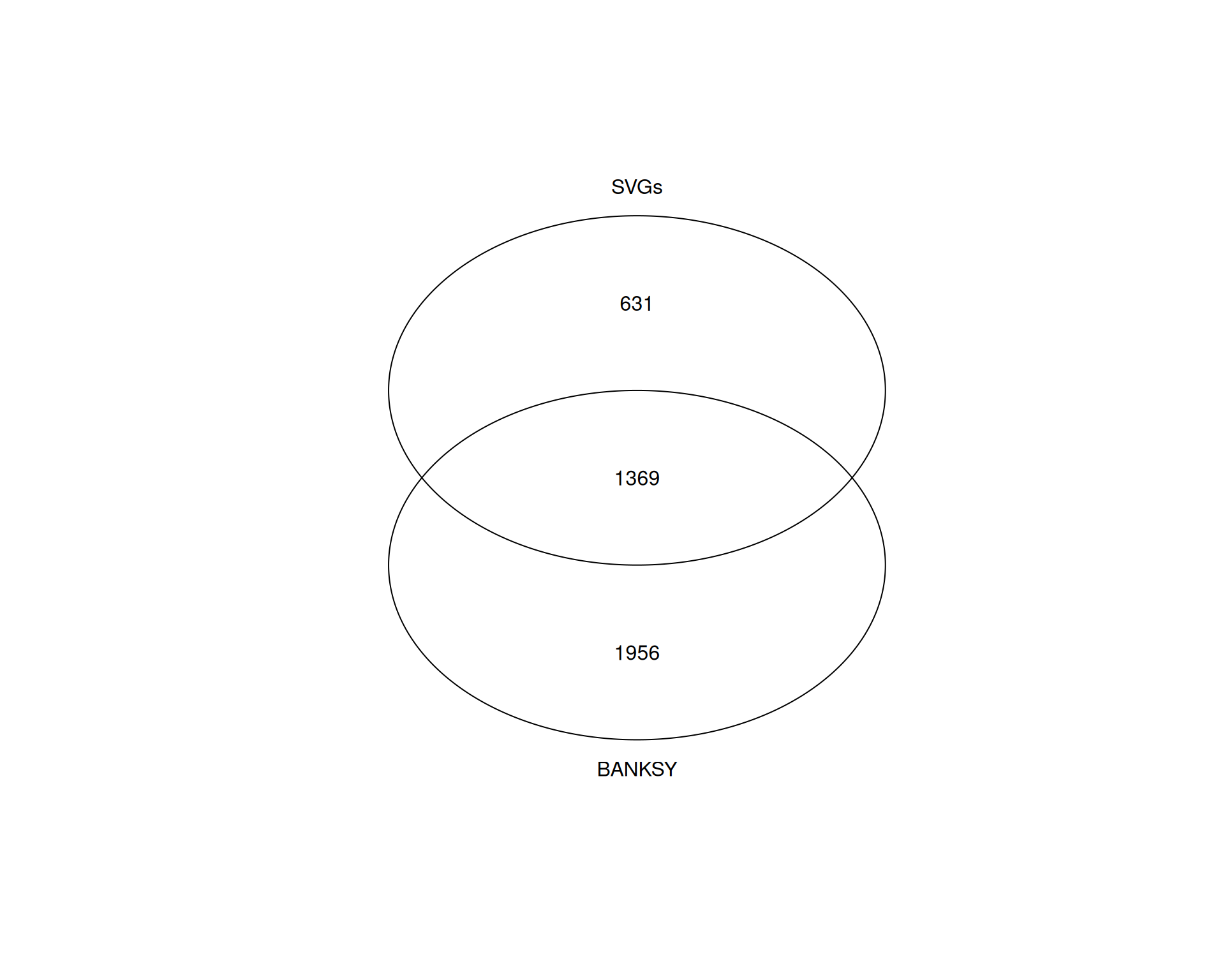
Approximately 70% of the SVGs are also identified as BANKSY marker genes, but many BANKSY markers are not among the SVGs.
Again, we emphasise that this doesn’t mean one method is superior, as they capture different aspects of spatial organisation. SVGs are selected based on spatial variability across the tissue: high expression in some locations, low in others. BANKSY markers are selected based on differential expression between spatially informed clusters.
The overlap suggests BANKSY clusters capture genuine spatial patterns. BANKSY markers not identified as SVGs may reflect cell identity markers within spatially defined domains or fine-scale spatial patterns not captured by SVG methods.
Conversely, non-spatial clustering may identify cell type clusters that are not spatially organised or sparsely distributed across regions (for example, scattered immune cells in tumour tissue), which BANKSY might miss because spatial coherence is prioritised, merging them with surrounding tissue.
11.5 Export the Seurat Object
As usual, it’s a good idea to save your intermediate file for future use:
saveRDS(visium, "results/mouse_brain_banksy.rds")11.6 Exercises
ExerciseExercise 1 - Exploring lambda
In the code above, we ran BANKSY with lambda = 0.2, which weights transcriptional information more heavily than spatial information. Try running BANKSY with lambda = 0.8, which weights spatial information more heavily, and compare the results.
To avoid overwriting the previous results:
- In
RunBanksy()use theassay_nameoption to name the new assay differently (e.g. “BANKSY_lambda_0.8”). - In
FindClusters()use thecluster.nameoption with a different name (e.g. “banksy_cluster_lambda_0.8”).
AnswerAnswer
We adapt the workflow with the new lambda value and updated assay and cluster names. The names are intentionally verbose for clarity, though you may prefer shorter names in your own analysis.
# Run BANKSY
visium <- visium |>
  RunBanksy(
    assay = "SCT",
    lambda = 0.8,
    k_geom = 18,
    use_agf = TRUE,
    features = "all",
    assay_name = "banksy_lambda_08"
  )

# PCA, Clustering and UMAP
visium <- visium |>
  RunPCA(
    assay = "banksy_lambda_08",
    reduction.name = "pca_banksy_lambda_08",
    reduction.key = "pcabanksylambda08_",
    features = rownames(visium[["banksy_lambda_08"]]),
    npcs = 50
  ) |>
  FindNeighbors(reduction = "pca_banksy_lambda_08", dims = 1:50) |>
  FindClusters(cluster.name = "banksy_cluster_lambda_08", resolution = 0.8) |>
  RunUMAP(
    reduction = "pca_banksy_lambda_08",
    dims = 1:50,
    reduction.name = "umap_banksy_lambda_08"
  )
Modularity Optimizer version 1.3.0 by Ludo Waltman and Nees Jan van Eck
Number of nodes: 2780
Number of edges: 62709
Running Louvain algorithm...
Maximum modularity in 10 random starts: 0.8707
Number of communities: 16
Elapsed time: 0 seconds# Confirm the new assay and dimensionality reductions are present
Assays(visium)[1] "Spatial" "SCT" "Scran" "BANKSY"
[5] "banksy_lambda_08"Reductions(visium)[1] "pca" "umap" "tsne"
[4] "pca_banksy" "umap_banksy" "pca_banksy_lambda_08"
[7] "umap_banksy_lambda_08"We now plot these results alongside the lambda = 0.2 analysis:
# UMAP plot
banksy_umap_08 <- DimPlot(
  visium,
  reduction = "umap_banksy_lambda_08",
  group.by = "banksy_cluster_lambda_08",
  label = TRUE
) +
  ggtitle("lambda = 0.8, k_geom = 18") +
  theme_void()

# Spatial plot
banksky_spatial_08 <- SpatialDimPlot(
  visium,
  group.by = "banksy_cluster_lambda_08",
  label = TRUE,
  label.size = 4,
  image.alpha = 0.5
) +
  theme(legend.position = "none")

# Plot alongside the previous lambda = 0.2 results
(banksy_umap_08 + banksky_spatial_08) /
  (banksy_umap + banksky_spatial)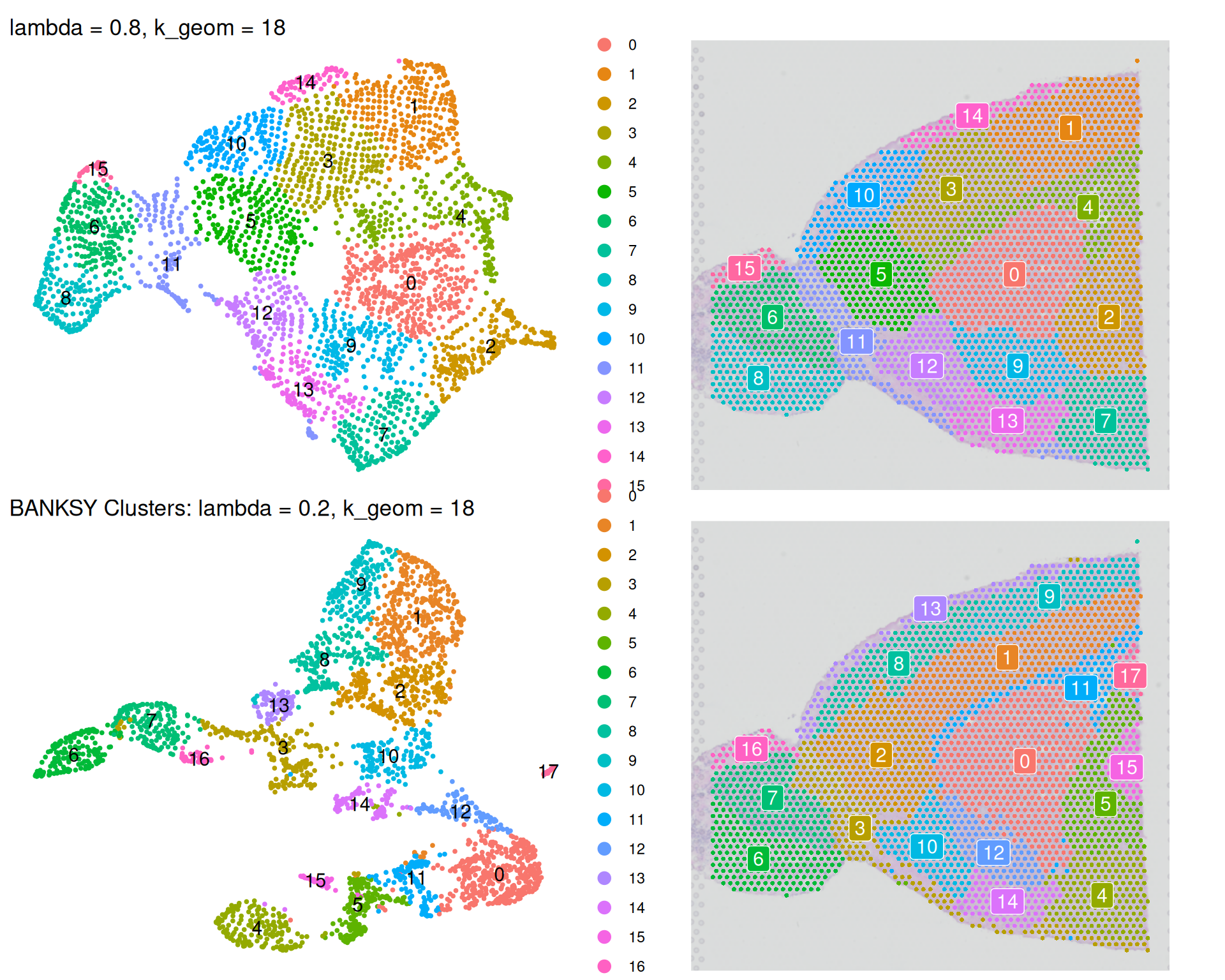
We can see some differences when comparing the analyses:
- The
lambda = 0.8analysis identifies fewer clusters thanlambda = 0.2, because clustering now prioritises spatial coherence over transcriptional similarity. Neighbouring tissue regions are more likely to be grouped together. - The
lambda = 0.8UMAP nearly recreates the original spatial tissue architecture when rotated 180 degrees. This demonstrates that higher lambda values drive clustering primarily by spatial information, producing clusters that closely reflect underlying tissue organisation.
Choose lambda based on your biological question. For identifying tissue domains defined by spatial context, use a higher lambda value. For identifying cell types that may be scattered across different regions, use a lower lambda value.
ExerciseExercise 2 - Exploring neighbourhood size
The parameter k_geom controls the number of nearest neighbours used to calculate spatially-augmented features. A larger value includes more neighbours and amplifies spatial information.
Run BANKSY with k_geom = 60, keeping lambda = 0.2 as in the original analysis. This includes four rings of spots on the hexagonal lattice (see discussion box above). Compare the results to the original analysis (lambda = 0.2, k_geom = 18).
AnswerAnswer
# Run BANKSY
visium <- visium |>
  RunBanksy(
    assay = "SCT",
    lambda = 0.2,
    k_geom = 60,
    use_agf = TRUE,
    features = "all",
    assay_name = "banksy_k_60"
  )

# PCA, Clustering and UMAP
visium <- visium |>
  RunPCA(
    assay = "banksy_k_60",
    reduction.name = "pca_banksy_k_60",
    reduction.key = "pcabanksyk60_",
    features = rownames(visium[["banksy_k_60"]]),
    npcs = 50
  ) |>
  FindNeighbors(reduction = "pca_banksy_k_60", dims = 1:50) |>
  FindClusters(cluster.name = "banksy_cluster_k_60", resolution = 0.8) |>
  RunUMAP(
    reduction = "pca_banksy_k_60",
    dims = 1:50,
    reduction.name = "umap_banksy_k_60"
  )
Modularity Optimizer version 1.3.0 by Ludo Waltman and Nees Jan van Eck
Number of nodes: 2780
Number of edges: 67581
Running Louvain algorithm...
Maximum modularity in 10 random starts: 0.8705
Number of communities: 14
Elapsed time: 0 seconds# Confirm the new assay and dimensionality reductions are present
Assays(visium)[1] "Spatial" "SCT" "Scran" "BANKSY"
[5] "banksy_lambda_08" "banksy_k_60" Reductions(visium)[1] "pca" "umap" "tsne"
[4] "pca_banksy" "umap_banksy" "pca_banksy_lambda_08"
[7] "umap_banksy_lambda_08" "pca_banksy_k_60" "umap_banksy_k_60" We create UMAP and spatial plots for this analysis and compare them to the original:
# UMAP plot
banksy_umap_k60 <- DimPlot(
  visium,
  reduction = "umap_banksy_k_60",
  group.by = "banksy_cluster_k_60",
  label = TRUE
) +
  ggtitle("Lambda = 0.2, k_geom = 60") +
  theme_void()

# Spatial plot
banksky_spatial_k60 <- SpatialDimPlot(
  visium,
  group.by = "banksy_cluster_k_60",
  label = TRUE,
  label.size = 4,
  image.alpha = 0.5
) +
  theme(legend.position = "none")

# Plot alongside the previous results
(banksy_umap_k60 + banksky_spatial_k60) /
  (banksy_umap + banksky_spatial)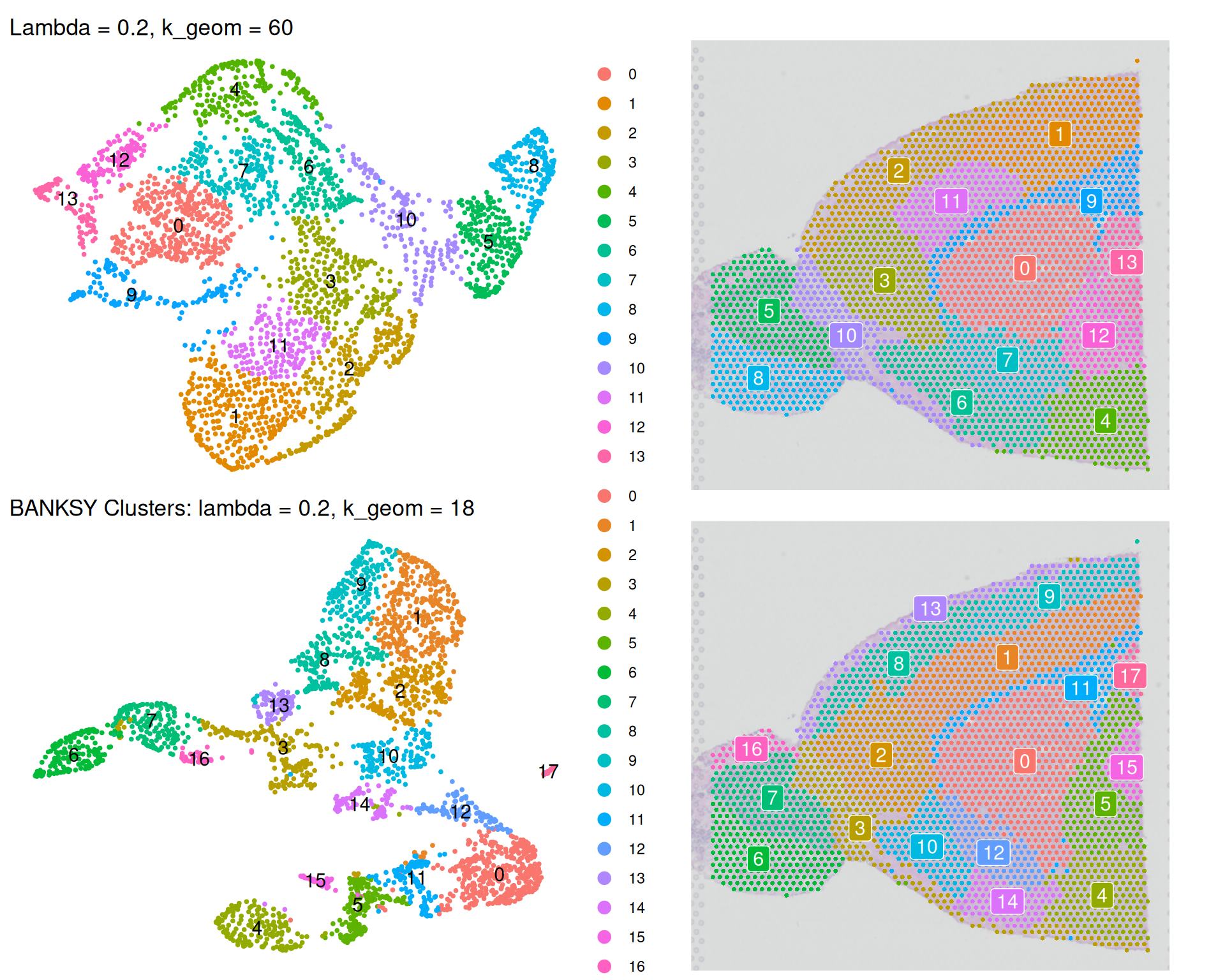
Increasing k_geom to 60 results in:
- Fewer clusters are identified because the larger neighbourhood creates a more connected graph, merging smaller spatial regions into larger domains.
- The UMAP more closely reflects the original tissue architecture because the larger spatial neighbourhood emphasises spatial coherence in clustering.
This effect is similar to increasing lambda. However, note the two parameters are different:
- With
k_geomwe’re controlling the size of the neighbourhood over which BANKSY calculates its spatial expression metrics. - With
lambdawe control how much weight we put on those spatial expression features, compared to the original expression values.
Choose k_geom based on your assumptions about tissue domain size. Lower values are appropriate for data with finely structured tissue. Higher values smooth over fine structure and identify larger domains.
For Visium v1/v2 data (like our dataset), each spot already measures averaged expression from multiple cells. This implicitly incorporates spatial information. You may therefore want to use lower k_geom and lambda values than for high-resolution technologies such as Visium HD and Xenium.
11.7 Summary
TipKey Points
- Use
RunBanksy()to augment expression data with spatial features: mean neighbourhood expression (average expression in neighbouring spots) and azimuthal Gabor filter (directional changes in expression).RunBanksy()has three key parameters:lambda(balance between spatial and transcriptional information),k_geom(number of spatial neighbours), anduse_agf(whether to calculate AGF features).- The resulting augmented matrix has three times as many features as the original: original expression plus two spatial features per gene.
- BANKSY clusters differ from non-spatial clusters because they prioritise spatial coherence alongside transcriptional similarity.
- Non-spatial clustering identifies cell identities: cells with similar expression profiles, regardless of location.
- BANKSY identifies tissue domains: spatially coherent regions defined by both expression and spatial context, which may contain multiple cell types.
- Visualising both methods side-by-side reveals how BANKSY fragments scattered clusters into spatially unified regions.
- BANKSY marker genes overlap substantially with spatially variable genes (SVGs) but may include additional markers reflecting cell identity within spatial domains.
- BANKSY markers not identified as SVGs may reflect uniform expression within a domain or cell type identity within a spatial region.
- Non-spatial clustering and spatial analysis are complementary to each other.
- Adjust
lambdaandk_geomto control the balance between spatial coherence and transcriptional similarity.- Higher
lambda(e.g. 0.8) emphasises spatial coherence, identifying larger tissue domains. - Lower
lambda(e.g. 0.2) emphasises transcriptional similarity, allowing cell types to be identified across multiple spatial regions. - Higher
k_geomincreases neighbourhood size and spatial smoothing, resulting in fewer and larger clusters. - Lower
k_geomcreates more fragmented neighbourhoods, identifying finer tissue structure.
- Higher
- The choice of
lambdaandk_geomis critically dependent on the resolution of your spatial technology.- For Visium v1/v2 data, lower values work well because each spot already averages multiple cells’ expression.
- For higher resolution technologies, higher values may be beneficial to detect larger tissue domain organisations.