Describe the main spatial transcriptomics package ecosystems available in R and Python.
Load Visium data into Seurat with Load10X_Spatial().
Inspect the main components of a Seurat object, including assays, metadata, and images.
Visualise spatial data with Seurat plotting functions.
Save a Seurat object to disk and reload it with saveRDS() and readRDS().
4.1 Choosing a package ecosystem
Several software packages are available for spatial transcriptomics analysis, but they do not all use the same data structure. Broadly speaking, there are three ecosystem families:
Seurat (R): A popular package suite for single-cell, spatial, and multi-omic analysis. It provides a single, integrated workflow around the Seurat object.
Bioconductor (R): Rather than a single package, Bioconductor provides the SpatialExperiment object, and package developers build analysis tools around it. The SpatialExperiment object is compatible with SingleCellExperiment, so it also works with packages designed for single-cell and multi-omic data. The Orchestrating Spatial Transcriptomics Analysis with Bioconductor (OSTA) book is a fantastic reference for this ecosystem.
scverse (Python): This project brings together several Python packages for single-cell, spatial, and multi-omic analysis. squidpy provides spatial analysis functionality with AnnData as the main data structure. More recent work has introduced the SpatialData object and package, which squidpy can also use.
Choosing between ecosystems is not always straightforward. They all cover the same core tasks, such as filtering, clustering, and dimensionality reduction, but individual algorithms may be available in only one ecosystem. Performance can also differ between packages, especially for very large datasets.
One way to approach this is to choose one ecosystem as your main working environment and become comfortable with its object structure. And then switch when a particular method or dataset requires it. In these materials, we use Seurat because it is the package some of the authors know best. The same conceptual steps, however, apply across the other ecosystems.
NoteObject format conversion
When you move between ecosystems, you can convert objects in two main ways:
Manually create the new object from the components of the old one. For example, you can use the raw count matrix and metadata from a Seurat object to build a SingleCellExperiment object. While flexible, this requires familiarity with the target object.
Object definitions change over time, especially in Seurat. Always check that the converted object still looks as expected before you continue.
4.2 Loading Visium data
To load Visium data into Seurat, use the Load10X_Spatial() function. It expects two inputs:
the Space Ranger output directory, which should contain a spatial directory with the image data;
the corresponding filtered_feature_bc_matrix.h5 file, which contains the processed gene-by-spot matrix from Space Ranger.
The example below loads the Visium brain dataset used throughout the materials. We store it in an object called visium so that the variable name reflects the dataset.
# Load librarieslibrary(Seurat)library(paletteer) # for colour paletteslibrary(ggplot2)# Load the spatial transcriptomics datavisium <-Load10X_Spatial("data/mouse_sagittal_visium_v1",filename ="V1_Mouse_Brain_Sagittal_Anterior_Section_2_filtered_feature_bc_matrix.h5")# Inspect the class of the objectclass(visium)
[1] "Seurat"
attr(,"package")
[1] "SeuratObject"
This creates a Seurat object containing gene expression data, spatial coordinates, a tissue image, and associated metadata.
TipLoading data from other spatial technologies
Seurat also provides functions for other spatial technologies, such as LoadXenium() for 10x Genomics Xenium data and LoadVizgen() for Vizgen MerFISH data. Each function expects the file structure produced by its corresponding platform (e.g. Xenium Ranger).
4.3 Inspecting the Seurat object
The Seurat object contains several related data types together in one container. That makes it easier to keep expression data, metadata, images, and analysis results aligned as you move through the workflow.
The main components are:
assays: Contains the gene expression data as a matrix of genes (rows) by spots/cells (columns).
Each assay may contain different layers (matrices), such as raw and normalised counts.
Multiple assays may also be present, for example to store different types of data (e.g. gene expression, protein expression) or transformations over the original data.
meta.data: Contains metadata for each spot/cell, such as quality control metrics and experimental conditions.
reductions: Contains dimensionality reduction results, such as PCA or UMAP.
images: Contains images associated with the spatial transcriptomics data.
graphs: Contains graph-based representations of the data, such as nearest neighbour graphs.
tools: Contains various tools and methods used for analysis.
The Seurat manual provides a detailed list of accessors for these components. We will use several of them throughout the materials, but for now we will focus on assays and metadata because you will use them most often at this stage.
4.3.1 Assays
Seurat uses the Default Assay to identify the active assay that functions use by default. You can list all assays in an object with:
# List the assays present in the objectAssays(visium)
[1] "Spatial"
At the moment, the object contains only one assay, but later sections will add more. You can also use DefaultAssay() to check which assay is currently active. For Visium data, the default assay is called "Spatial" and contains the raw counts.
You can access assays by name with double-bracket notation [["AssayName"]]:
# Access the default assayvisium[["Spatial"]]
Assay (v5) data with 32285 features for 2823 cells
First 10 features:
 Xkr4, Gm1992, Gm19938, Gm37381, Rp1, Sox17, Gm37587, Gm37323, Mrpl15,
Lypla1
Layers:
 counts
In this case, the assay contains a single layer called counts. That layer stores the raw count matrix, which you can inspect directly:
# Access the counts matrixvisium[["Spatial"]]$counts
The counts are stored as a sparse matrix, which is an efficient format for matrices with many zeros. In the printed output, zeros appear as .. That pattern is normal for spatial count data, where most genes are not detected in most spots.
4.3.2 Metadata
An important part of the object is the metadata for each spot or cell. You can access it with empty double square brackets [[]]:
This is stored as a regular R data.frame and by default contains:
Row names, which identify each spot or cell.
orig.ident, which records where the data came from if the object contains more than one dataset. By default, Seurat sets this to "SeuratProject".
nCount_Spatial and nFeature_Spatial, which store the total counts and detected genes for each spot. We will use these values again later.
You can access individual metadata columns with the $ accessor. For example:
# Get a numeric summary of the total spot countssummary(visium$nCount_Spatial)
   Min. 1st Qu.  Median    Mean 3rd Qu.    Max.
    207   14381   20152   20724   26794   61430
You can also add new metadata columns with the <- assignment operator. For example, the code below creates a logical column that records whether each spot has more than 1000 counts:
# Add a new column indicating whether the total counts are greater than 1000visium$nCountGreater1000 <- visium$nCount_Spatial >1000
TipFull object structure
Use str() when you want to inspect the full structure of the Seurat object:
# Explore the Seurat objectstr(visium)
4.3.3 Images
You can list the images stored in the object with:
# List the images present in the objectImages(visium)
[1] "slice1"
By default, the image data is called "slice1", although other datasets may use a different name. You can access the image-related data with the same double-bracket notation used for assays:
This returns an object of class VisiumV2, which contains the image data and associated metadata.
You usually do not interact with this object directly. Instead, Seurat uses it behind the scenes when you create spatial plots or run spatial analyses.
4.4 Visualising spatial data
Seurat provides several functions for visualising the spatial distribution of spots or cells and their associated features on the tissue slide.
The main functions are:
SpatialFeaturePlot() overlays continuous data on top of a spatial image. The input can be gene expression or a numeric metadata column.
SpatialDimPlot() is the categorical equivalent.
ImageFeaturePlot() and ImageDimPlot() use the same data, but they show only the spots and not the tissue image.
The examples below show transcript counts, a simple metadata category, and the same data without the image background. This helps you see how the different plot types emphasise different aspects of the same object.
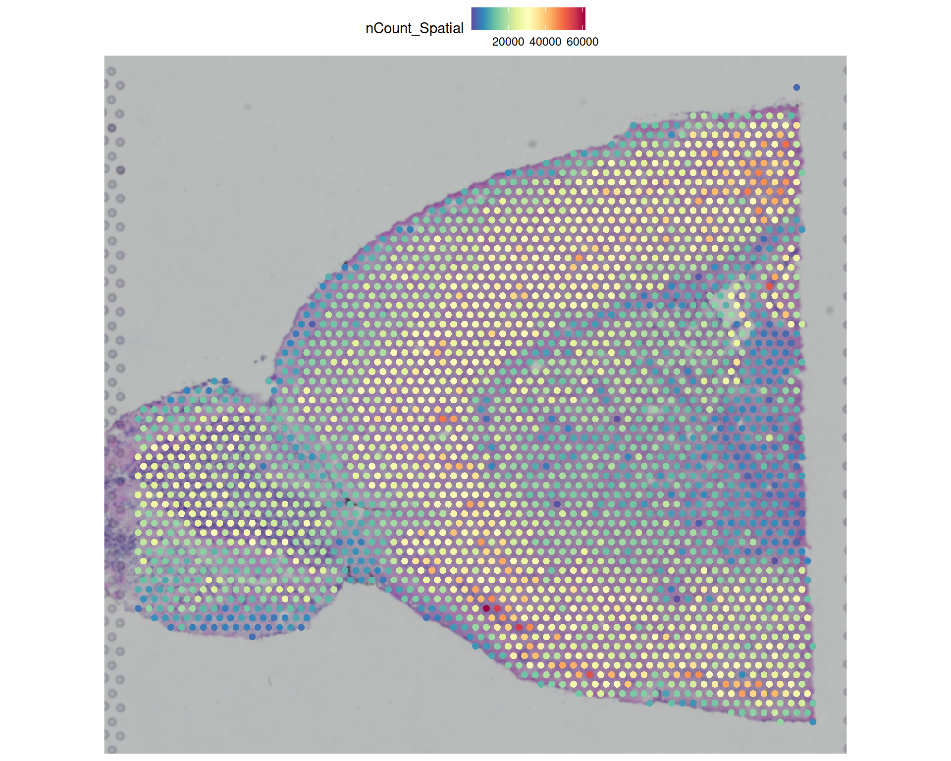
# Visualise the number of transcripts per spotSpatialFeaturePlot(visium, features ="nCount_Spatial")
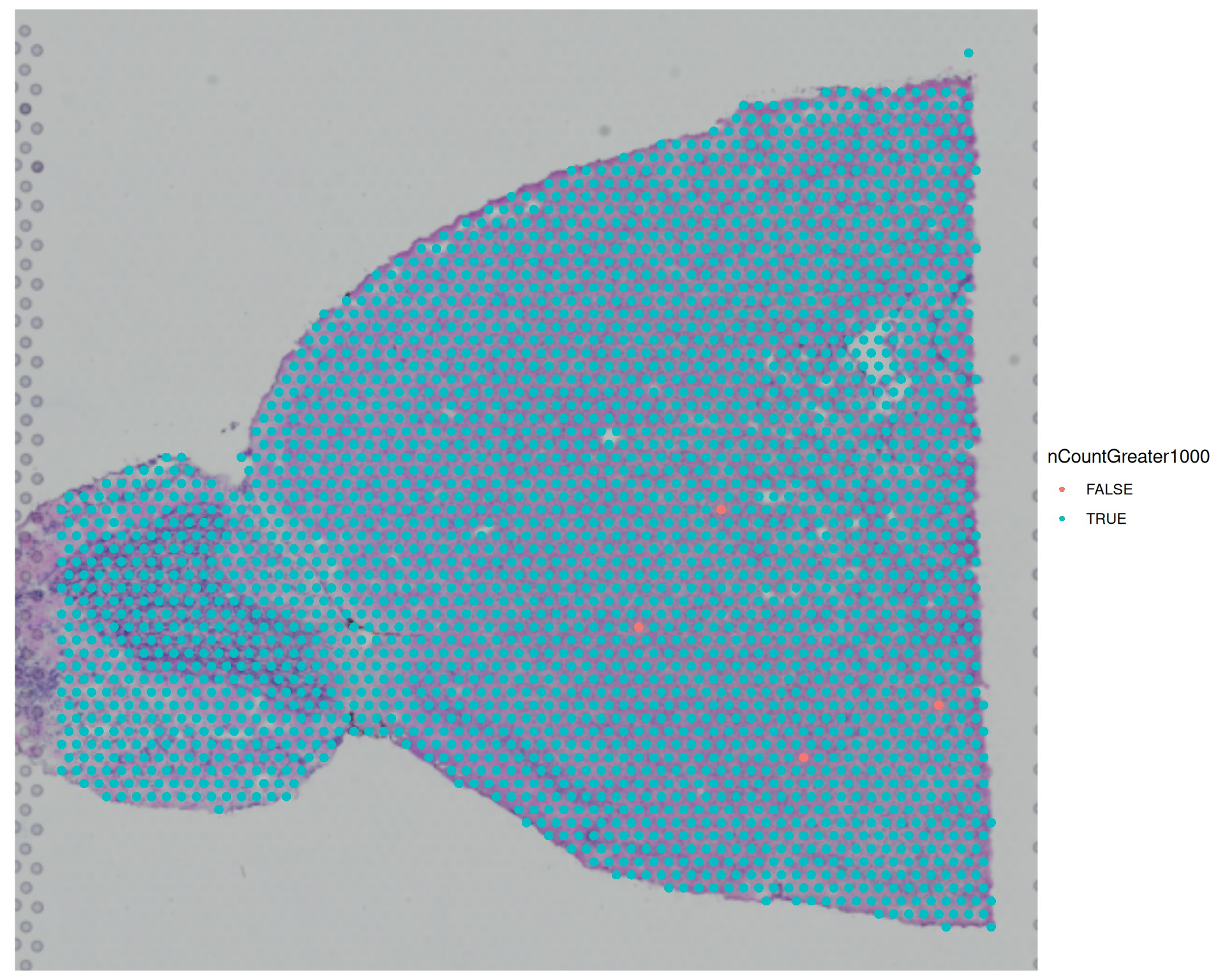
# Visualise the yes/no variable we created earlierSpatialDimPlot(visium, group.by ="nCountGreater1000")
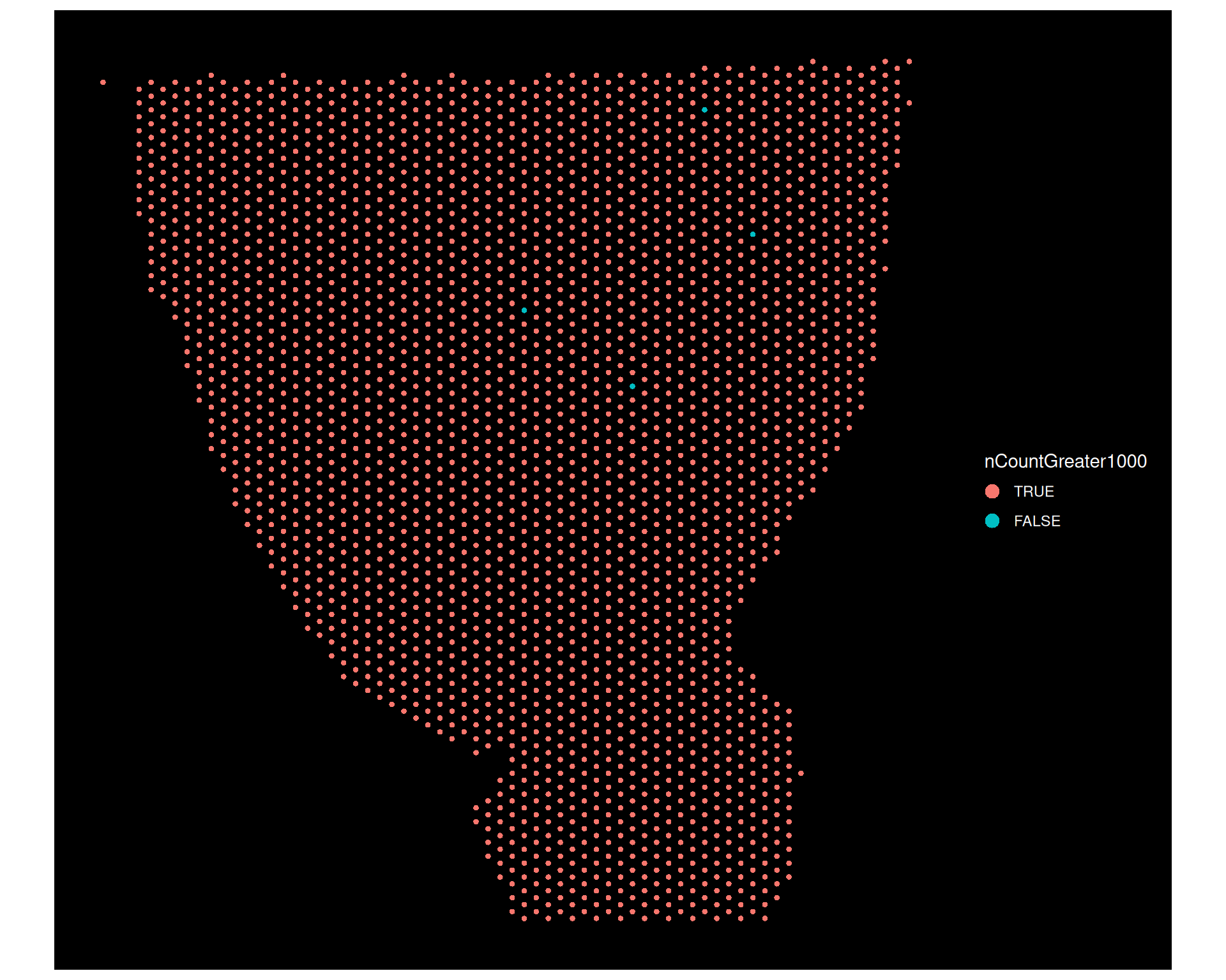
# Visualise the transcript locations on the tissue slide# size controls the size of the points (0.5 by default)ImageDimPlot(visium, group.by ="nCountGreater1000", size =1.5)
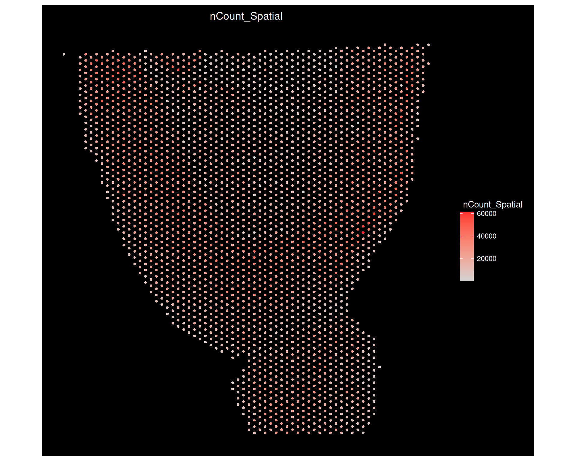
# Total counts againImageFeaturePlot(visium, features ="nCount_Spatial", size =1.5)
These functions return ggplot2 objects, so you can add further ggplot2 layers on top of them. For example, you can add a title to a spatial plot:
# Add title to the plotSpatialFeaturePlot(visium, features ="nCount_Spatial") +ggtitle("Total number of counts per spot")
4.5 Saving and reloading Seurat objects
Spatial analysis can be computationally demanding, so it is a good idea to save objects at intermediate steps and reload them later. That way, you do not need to repeat the previous analysis steps every time you return to the project.
You can do this with the standard R functions saveRDS() and readRDS(), which save and load R objects in a binary format.
# Save the Seurat object to disksaveRDS(visium, file ="results/visium_brain.rds")
To re-read the object later on, you can use:
# Load the Seurat object from diskvisium <-readRDS("results/visium_brain.rds")
4.6 Loading Xenium Data
If you are working with 10X Genomics Xenium data, you can use the LoadXenium() function to load the data into a Seurat object. This function is specifically designed to handle the unique structure of Xenium data, which includes spatial transcriptomics data with high-resolution spatial coordinates and associated images.
We will use another dataset from the 10X examples. The data is available on the 10X website and has been downloaded for you in the course materials at data/human_melanoma_xenium.
# load the xenium data - takes a while to loadxenium <-LoadXenium("data/human_melanoma_xenium", fov ="fov")
The FOV (Field of View) parameter allows you to specify which field of view to load if the dataset contains multiple fields. In this case, we are loading the default field of view.
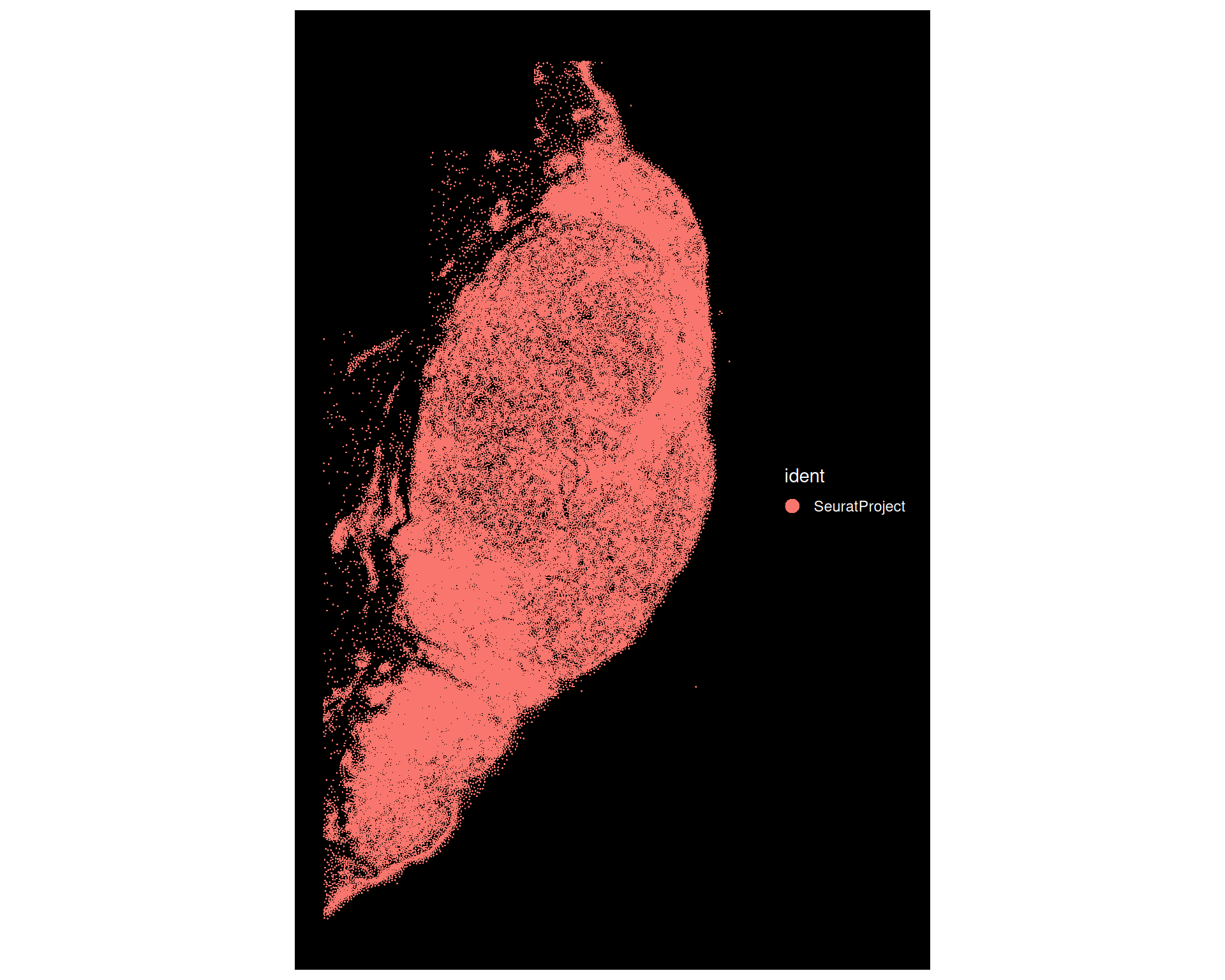
For single-cell resolution methods like Xenium, we can use the ImageDimPlot() function to plot the spatial distribution of cells or spots in the tissue slide:
# Visualise the locations of the transcripts on the tissue slideImageDimPlot(xenium)
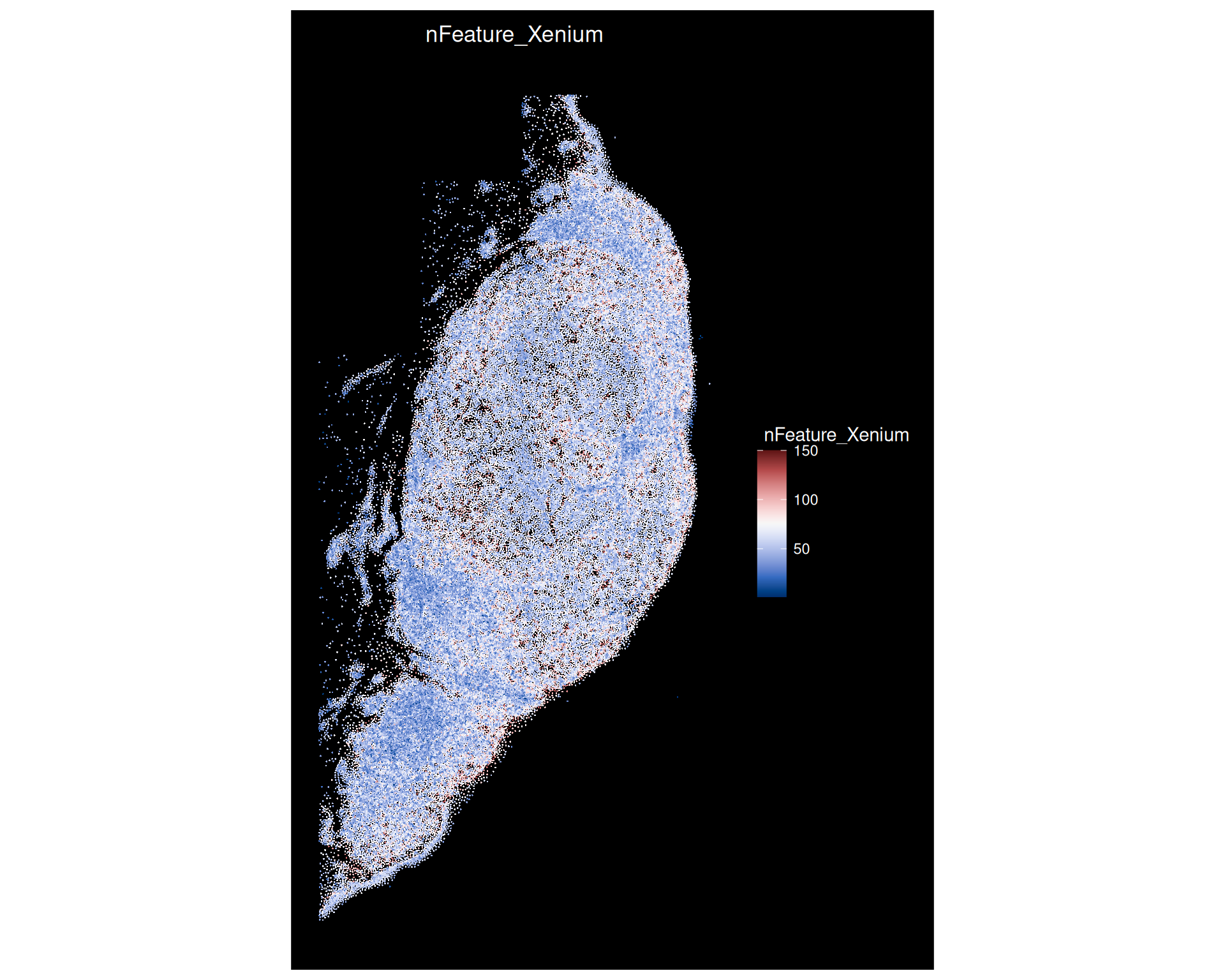
We can also visualise the number of features measured in each location using ImageFeaturePlot():
# Visualise the transcript density on the tissue slideImageFeaturePlot( xenium,features ="nFeature_Xenium",cols =paletteer_c("grDevices::Blue-Red 3", 150))
This shows that while the spatial resolution is very high, the number of features measured per location is low compared to other spatial transcriptomics technologies. In this case only 382 genes were measured, and the visualisation above shows the scale only going up to a maximum of 150 features detected per position.
We can compare the range of features detected between the two technologies here:
# Summary of number of detected featuressummary(xenium$nFeature_Xenium)
   Min. 1st Qu.  Median    Mean 3rd Qu.    Max.
   3.00   44.00   56.00   57.12   69.00  150.00
summary(visium$nFeature_Spatial)
   Min. 1st Qu.  Median    Mean 3rd Qu.    Max.
    166    4270    5342    5173    6231    8689
Xenium datasets can be quite large, so make sure you have enough memory available to load the data. If you encounter memory issues, consider using a machine with more RAM or using a subset of the data for analysis.
4.7 Example MERFISH file
As an example, we provide a pre-processed MERFISH file of the Human heart, which has been saved as a Seurat object:
# Load the preprocessed MERFISH datasetmerfish <-readRDS("data/human_heart_merfish/overall_merfish.rds")# Examine the objectmerfish
An object of class Seurat
238 features across 228635 samples within 1 assay
Active assay: RNA (238 features, 0 variable features)
 2 layers present: counts, data
 3 dimensional reductions calculated: pca, umap, spatial
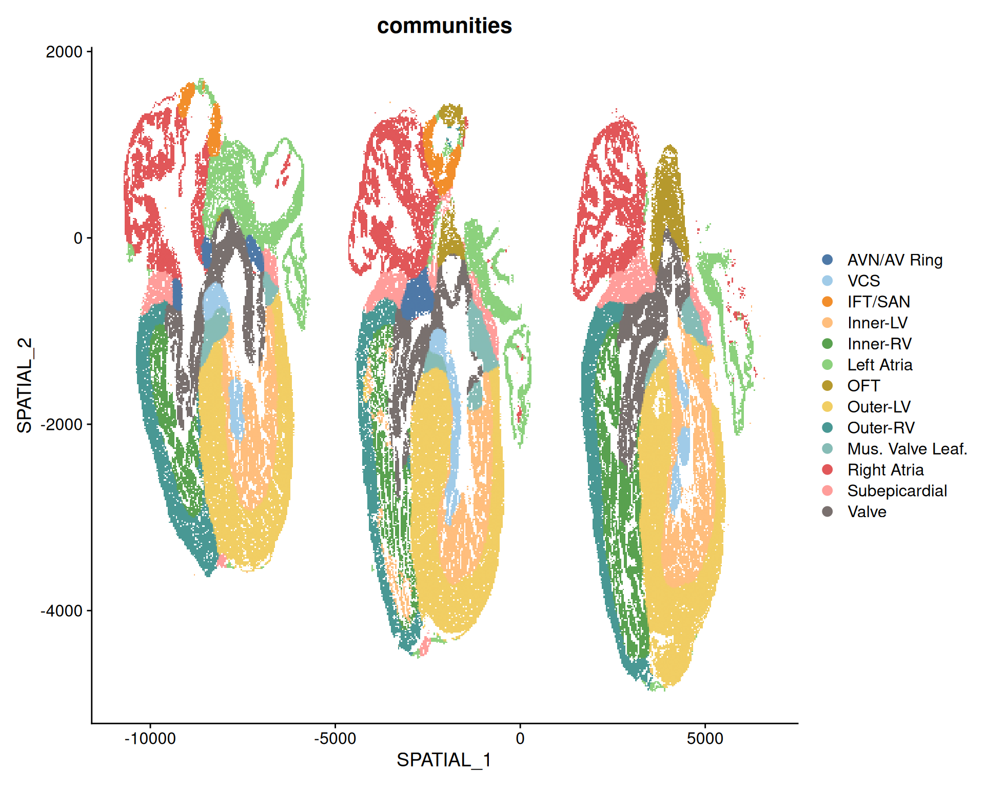
MERFISH data does not have an associated image with it, and is stored as if it was a single-cell dataset. The spatial information is represented as a dimensionality reduction slot, which we can visualise with the DimPlot() function.
# Visualize the structure of the heart in the MERFISH dataDimPlot( merfish,reduction ="spatial",group.by ="communities",cols =paletteer_d("ggthemes::Tableau_20"))