# Load libraries
library(Seurat) # single-cell and spatial analysis toolkit
library(sparseMatrixStats)
library(paletteer) # colour palettes
library(ggplot2) # plotting
library(dplyr) # data manipulation
library(patchwork) # combining plots

# Load the Seurat object from the previous chapter
visium <- readRDS("precomputed/mouse_brain_visium_deconvolution.rds")13 Cell-Cell Communication
TipLearning Objectives
- Explain how cell-cell communication can be inferred from ligand-receptor expression patterns in spatial transcriptomics data.
- Create a
CellChatobject from a Seurat object and prepare the spatial inputs it needs. - Select and subset a suitable ligand-receptor database for analysis.
- Compute communication probabilities and pathway-level scores with
CellChatand produce visualisations from these results. - Describe the main limitations of CCC analysis.
13.1 Setup
We continue working with the sagittal mouse brain dataset from previous chapters.
NoteClick to expand
Start by loading the required libraries and the Seurat object.
As a reminder, this object was created by:
- Importing the raw data using
Load10X_Spatial(), followed by QC and filtering to remove low-quality spots. - Data normalisation using
SCTransform(), which models technical variation and applies variance stabilisation. Stored in the “SCT” assay. - Applying dimensionality reduction using PCA, UMAP and t-SNE.
- Clustering the data using graph-based clustering. The clusters we use in this chapter were generated using the Leiden algorithm at a resolution of 0.8 and were set the the default cell identities (
Idents(visium)). - Identifying spatially variable features using Moran’s I and markvariogram methods.
- Running the BANKSY algorithm to identify spatial domains in the data, which were stored in the
banksy_clusterscolumn of the metadata. - Using the RCTD package to perform deconvolution of the spatial transcriptomics data, using a single-cell RNA-seq reference dataset of the mouse brain.
13.2 Overview
Cells in multicellular tissues communicate to coordinate development, immune responses and disease progression. One common communication mechanism involves signalling molecules (ligands) produced by one cell and detected by receptors on another cell. Receptor-mediated pathways can then influence gene expression, cell behaviour and cell fate decisions.
Single-cell and spatial transcriptomics let us study these interactions by measuring gene expression across many cells at once. Cell-cell communication analysis (CCC) uses curated ligand-receptor pairs to infer which signalling relationships are most likely between cell populations. The basic idea is that cells expressing a ligand are potential senders, and cells expressing the matching receptor are potential receivers. That makes it possible to build an interaction network and form hypotheses about how information moves through a tissue.
CCC methods do not discover new signalling pathways. They rely on curated databases of known ligand-receptor interactions and use the observed expression patterns to identify which of those interactions are most plausible in the data.
Spatial transcriptomics adds location information to this analysis. That helps because many signalling processes act locally, so sender and receiver cells are more plausible when they are near one another in the tissue. We can therefore ask how cell types communicate within the tissue microenvironment, not just whether they express compatible ligands and receptors.
Many packages now support cell-cell communication analysis from single-cell and spatial transcriptomics data. As with much of spatial analysis, this is an active area of development, so it is worth checking benchmark studies regularly. For example, Ku et al. 2026 compared several spatial and non-spatial CCC methods across multiple spatial transcriptomics technologies.
Their main conclusion was that there is no single best method for all datasets. Performance depends on spatial resolution, cell type composition and the assumptions of the methods. In general, methods designed for single-cell data perform well on high-resolution spatial datasets, while spatially aware methods can provide complementary information for lower-resolution technologies.
We discuss caveats and limitations at the end of the chapter. For now, we will use CellChat, a popular package for CCC analysis that was originally developed for single-cell data and is now used for spatial data as well. The benchmark study above used CellChat v2, which is also the version we use here. SpatialCellChat (aka CellChat v3) is under development and adds more spatial functionality.
TipAcronyms used in this chapter
Throughout this chapter we use the term cell-cell communication (CCC) to describe signalling relationships inferred from ligand-receptor expression patterns. The literature also frequently uses the term cell-cell interaction (CCI), and the two terms are often used interchangeably in the context of transcriptomics-based analyses.
13.3 CellChat Analysis
CellChat is an R package for inferring cell-cell communication networks from single-cell and spatial transcriptomics data. It combines gene expression measurements with a curated database of ligand-receptor interactions to estimate the probability of communication between cell populations. It also accounts for multi-subunit receptor complexes, cofactors and pathway-level organisation, which improves performance compared with methods that only use ligand-receptor pairs.
The analysis involves the following steps:
- Create the CellChat object
- Set the ligand-receptor interaction database
- Identify variable genes and interactions
- Compute communication probabilities and infer signalling pathways
- Visualise and explore the results
We will work through each step in turn. First, load the package:
# Load CellChat library
library(CellChat)
13.3.1 Create CellChat Object
You can create the CellChat object directly from a Seurat object with createCellChat().
In spatial mode, this function also needs a data frame of spatial conversion factors with two columns:
ratio: the conversion factor that turns spatial coordinates from pixels into microns. For example, a ratio of 0.1 means that 1 pixel equals 0.1 μm.tol: a tolerance factor that gives CellChat some flexibility when it calculates interaction ranges. The authors recommend setting this to half the spot diameter in microns.
The ratio value can be calculated from the spatial resolution of the data. It is the spot diameter in microns divided by the spot diameter in pixels. The spot diameter in pixels is stored as image metadata, and you can obtain the image list in a Seurat object with Images().
# View scale factors for the image in the Seurat object
ScaleFactors(visium[["slice1"]])
$spot
[1] 89.47248
$fiducial
[1] 144.5325
$hires
[1] 0.172117
$lowres
[1] 0.05163511
attr(,"class")
[1] "scalefactors"The spot entry is the one we need here. It gives the number of pixels corresponding to the spot diameter, which is 55 μm for 10X Visium v1/v2.
We can now create the spatial factors data frame:
# Create spatial factors data frame
spatial_factors <- data.frame(
  ratio = 55 / ScaleFactors(visium[["slice1"]])$spot,
  tol = 55 / 2
)

spatial_factors
ratio tol
1 0.6147141 27.5CellChat also needs a data frame with the spatial coordinates of each spot. We can extract those coordinates from the Seurat object with GetTissueCoordinates().
# Extract tissue coordinates of the spots
spatial_coords <- GetTissueCoordinates(visium, image = "slice1")[, c("x", "y")]

head(spatial_coords)
x y
AAACAAGTATCTCCCA-1 8599 7608
AAACACCAATAACTGC-1 2886 8686
AAACAGAGCGACTCCT-1 8048 3297
AAACAGCTTTCAGAAG-1 2198 6770
AAACAGGGTCTATATT-1 2473 7249
AAACATTTCCCGGATT-1 8255 8926Before creating the CellChat object, it is worth checking the spot distances that CellChat will use. For 10X Visium v1, the minimum distance should be roughly 100 μm between the centres of adjacent spots, so this is a useful sanity check on the spatial conversion factors.
# compute distances of the spots to each other
spot_dists <- computeCellDistance(
  coordinates = spatial_coords,
  ratio = spatial_factors$ratio,
  tol = spatial_factors$tol
)

# minimum distance observed
# remove zero distances (distance of a spot to itself)
min(spot_dists[spot_dists != 0])
[1] 84.21583The observed value is slightly below 100 μm, but it is close enough to suggest that the spatial factors are sensible.
With the scale factors and spatial coordinates prepared, we can create the CellChat object with createCellChat().
# Create CellChat object
cell_chat <- createCellChat(
  object = visium,
  assay = "SCT",
  group.by = "first_type",
  datatype = "spatial",
  coordinates = spatial_coords,
  spatial.factors = spatial_factors
)
[1] "Create a CellChat object from a Seurat object"
The `meta.data` slot in the Seurat object is used as cell meta information
Create a CellChat object from spatial transcriptomics data... Set cell identities for the new CellChat object
The cell groups used for CellChat analysis are L2_3_IT, L6_CT, L6_IT, L5_PT, L5_IT, Vip, Lamp5, Sst, Sncg, Serpinf1, Pvalb, Endo, Peri, L6b, NP, L4, Oligo, Meis2, Astro, Macrophage, VLMC, SMC # drop levels of cell type labels that are not present in the data
cell_chat@idents <- droplevels(cell_chat@idents)The important options here are:
assay = "SCT": CellChat needs log-normalised expression data. We use the log-normalised data from theSCTransform()workflow, which are stored in theSCTassay. You could also useassay = "Spatial"if you wanted to use the log-normalised data fromLogNormalize(), which are stored in that assay.datatype = "spatial": this tells CellChat that we are working with spatial transcriptomics data, so it can use the spatial coordinates and factors in the analysis.group.by = "first_type": this specifies the metadata column that contains the cell type labels. We use the first cell type label from the deconvolution results (first_typein the metadata). You could also choose a different label, such asbanksy_clustersorLeiden_08.- We also provide the spatial coordinates and factors prepared in the previous steps.
13.3.2 Ligand-receptor database
The choice of ligand-receptor interaction database is a key part of CCC analysis. It determines which interactions CellChat can consider, so it can affect the results substantially. CellChat provides three built-in databases: CellChatDB.mouse, CellChatDB.human and CellChatDB.zebrafish. For custom databases, you can use updateCellChatDB() and supply your own ligand-receptor pairs.
Here, we use the mouse database, which contains 3379 ligand-receptor interactions. We can quickly inspect the interaction categories available in this database:
# Visualise categories of interactions in the mouse database
showDatabaseCategory(CellChatDB.mouse)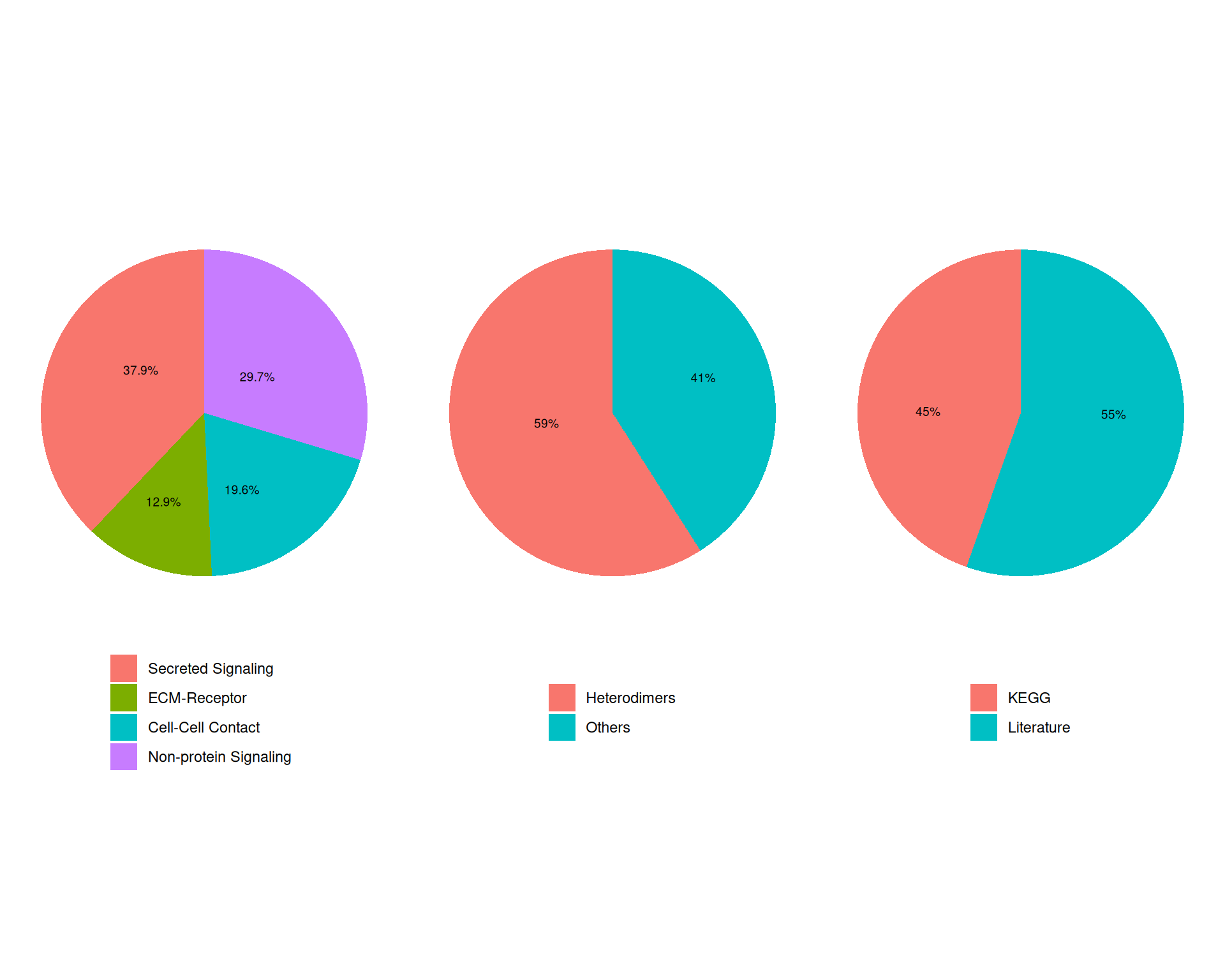
Each category corresponds to a different signalling mechanism that can occur between cells. In the next code chunk, we:
- Exclude the “Non-protein Signalling” category, which contains interactions that are not mediated by protein ligands and receptors.
- Add the filtered database to the CellChat object with the
@DBslot. - Use
subsetData()to keep only signalling genes from the database, which reduces the amount of data CellChat needs to process.
# Subset database to exclude "Non-protein Signalling"
mouse_db <- subsetDB(
  CellChatDB.mouse,
  search = c("Secreted Signaling", "ECM-Receptor", "Cell-Cell Contact"),
  non_protein = FALSE
)

# add the database to the CellChat object
cell_chat@DB <- mouse_db

# subset the expression data of signaling genes for saving computation cost
cell_chat <- subsetData(cell_chat)
We now have 922 genes available for the CCC analysis.
13.3.3 Variable Genes and Interactions
Before inferring the CCC network, CellChat identifies overexpressed genes in each group. This is effectively a differential expression test between the labels we defined above (first_type here), similar to the cluster marker genes analysis we performed earlier. CellChat then identifies ligand-receptor interactions where both partners are variable. Together, these steps focus the analysis on genes and interactions that are more likely to contribute to communication between cell populations.
# Identify overexpressed genes and interactions
cell_chat <- identifyOverExpressedGenes(cell_chat)
cell_chat <- identifyOverExpressedInteractions(cell_chat)
The number of highly variable ligand-receptor pairs used for signaling inference is 1168 This identifies 695 variable genes and 1168 variable ligand-receptor interactions.
13.3.4 CCC Network Inference
The final step is to compute communication probabilities for each ligand-receptor interaction and then infer the signalling pathways involved.
We start by computing the communication probability between cell groups with computeCommunProb().
# Compute communication probabilities
cell_chat <- computeCommunProb(
  cell_chat,
  contact.range = 100,
  interaction.range = 200
)
triMean is used for calculating the average gene expression per cell group.
[1] ">>> Run CellChat on spatial transcriptomics data using distances as constraints of the computed communication probability <<< [2026-06-11 16:17:57.417302]"
The input L-R pairs have both secreted signaling and contact-dependent signaling. Run CellChat in a contact-dependent manner for `Cell-Cell Contact` signaling, and in a diffusion manner based on the `interaction.range` for other L-R pairs.
[1] ">>> CellChat inference is done. Parameter values are stored in `object@options$parameter` <<< [2026-06-11 16:19:28.283659]"We set:
contact.range = 100to restrict contact-dependent interactions to a 100 μm radius. This matches the approximate distance between the centres of two adjacent 10X Visium spots. For single-cell resolution technologies, the recommendation is to use the average cell diameter instead.interaction.range = 200to restrict secreted signalling interactions to a 200 μm radius. The right value depends on the biological plausibility of medium-range interactions in the tissue as well as the spatial resolution of the data.
We can also compute communication probabilities at the signalling-pathway level with computeCommunProbPathway(). This function aggregates the probabilities of individual ligand-receptor interactions into pathway-level probabilities using the pathway structure in the database.
# Compute communication probabilities at the signaling pathway level
cell_chat <- computeCommunProbPathway(cell_chat)
Finally, we filter the inferred interactions so that we only keep those supported by a minimum number of cells. We also aggregate the resulting network, which we use in later visualisation steps.
# Filter interactions to only consider those supported by at least 10 spots
cell_chat <- filterCommunication(cell_chat, min.cells = 10)
The cell-cell communication related with the following cell groups are excluded due to the few number of cells: Sncg, Serpinf1 ! 0.8% interactions are removed!# Aggregate the communication network at the cell type level
cell_chat <- aggregateNet(cell_chat)The resulting CellChat object now contains the inferred interactions, their probabilities and the aggregated communication network between cell types.
13.4 CCC Network Visualisation
CellChat provides several ways to inspect the inferred cell-cell communication network.
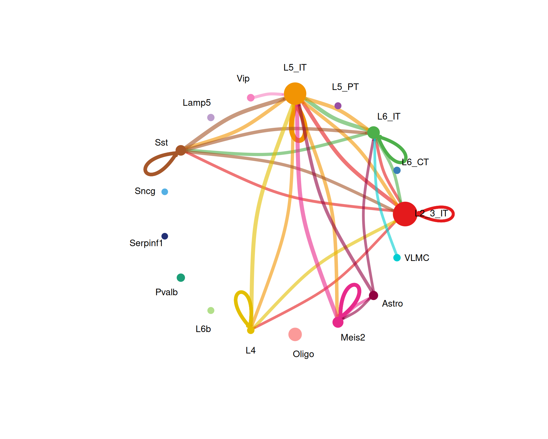
We start with the overall communication network using a circle plot. This shows the number of interactions and the summed interaction strength between cell types.
# calculate number of cells of each type for scaling the node sizes in the plot
group_size <- as.numeric(table(cell_chat@idents))

# Visualise the overall communication network as a circle plot
netVisual_circle(
  cell_chat@net$count,
  vertex.weight = group_size,
  weight.scale = TRUE,
  label.edge = FALSE,
  title.name = "Number of interactions",
  top = 0.1
)
# Visualise the weights of the interactions
netVisual_circle(
  cell_chat@net$weight,
  vertex.weight = group_size,
  weight.scale = TRUE,
  label.edge = FALSE,
  title.name = "Interaction weights/strength",
  top = 0.1
)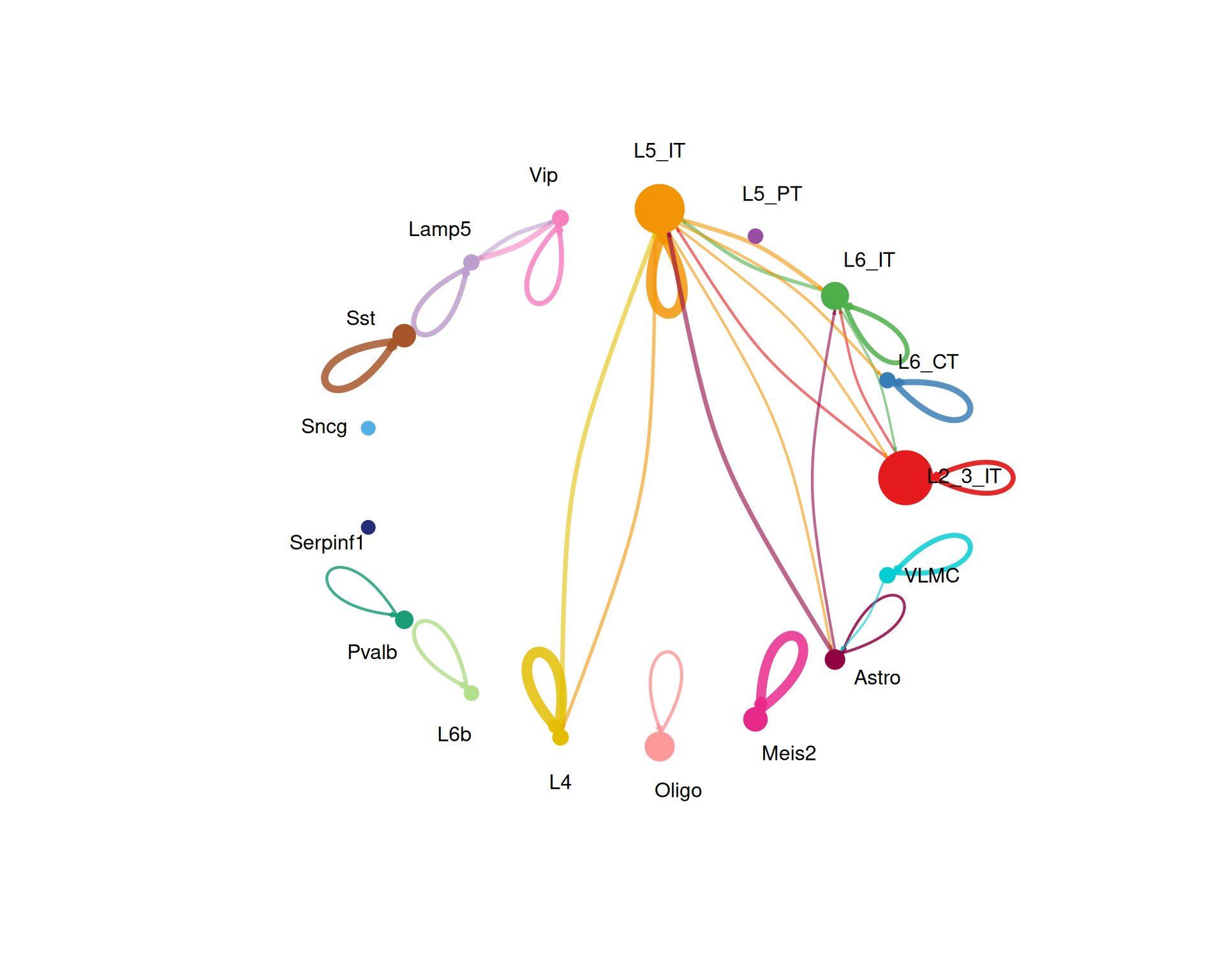
The top option keeps only the strongest 10% of interactions in the plot. You can increase or decrease this value depending on how cluttered the figure looks.
We can also visualise interaction strength as a heatmap:
# Visualise the interaction strength between cell types as a heatmap
netVisual_heatmap(cell_chat, measure = "weight")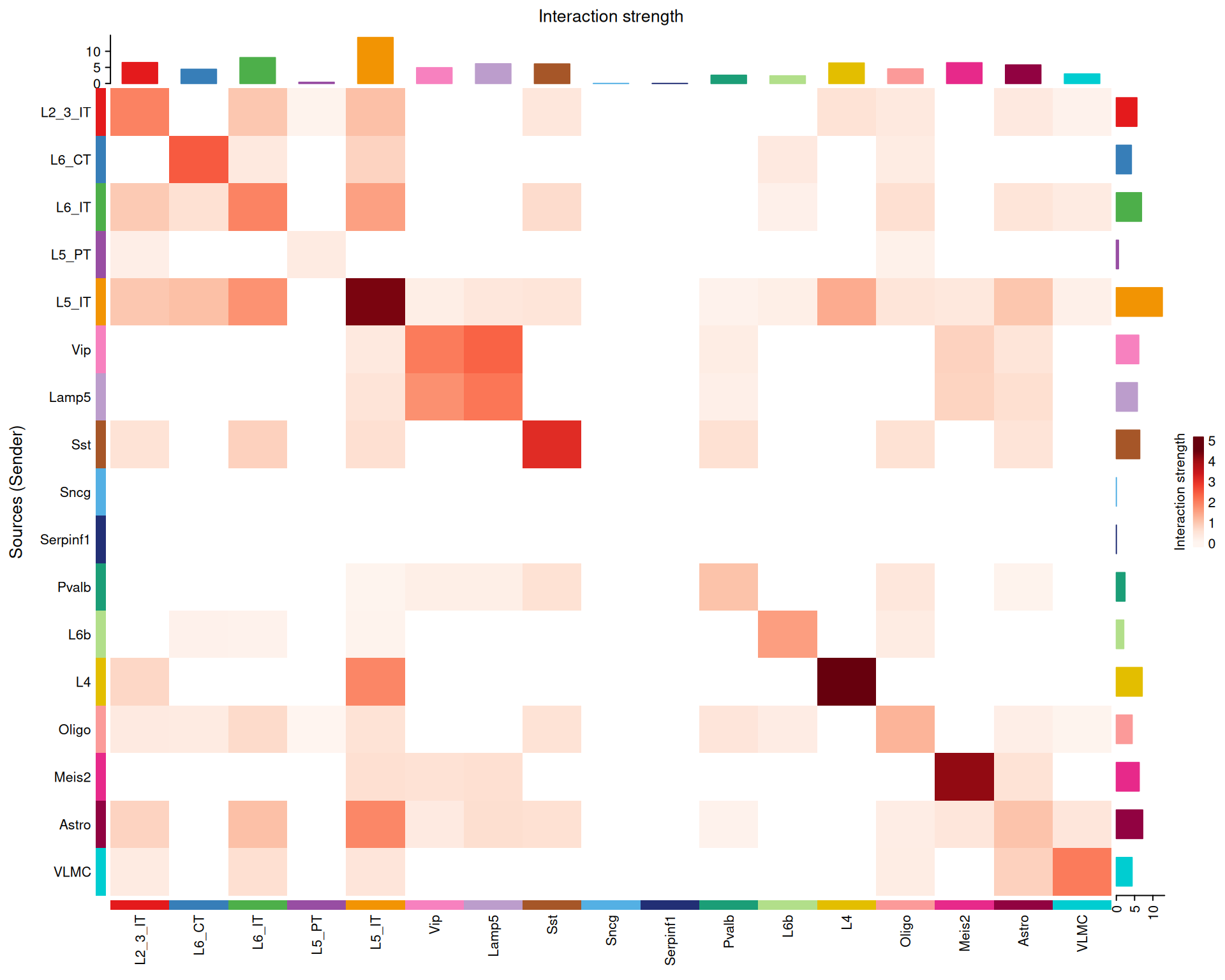
In general, the strongest interactions appear along the diagonal, where the same cell type communicates with itself. That is not surprising, because similar cells are often close to one another in the tissue and therefore more likely to interact.
There are also cross-type interactions. For example, Lamp5 → Vip appears in this dataset. If you want to check whether those cell types are nearby in the tissue, the next code block shows how to highlight their spatial locations.
Code for highlighting spatial locations of Lamp5 and Vip spots
# Highlight Lamp5 and Vip in side-by-side spatial plots
p1 <- SpatialDimPlot(
visium,
cells.highlight = WhichCells(visium, expression = first_type == "Lamp5"),
image.alpha = 0.5
) +
ggtitle("Lamp5 spot locations") +
theme(legend.position = "none")
p2 <- SpatialDimPlot(
visium,
cells.highlight = WhichCells(visium, expression = first_type == "Vip"),
image.alpha = 0.5
) +
ggtitle("Vip spot locations") +
theme(legend.position = "none")
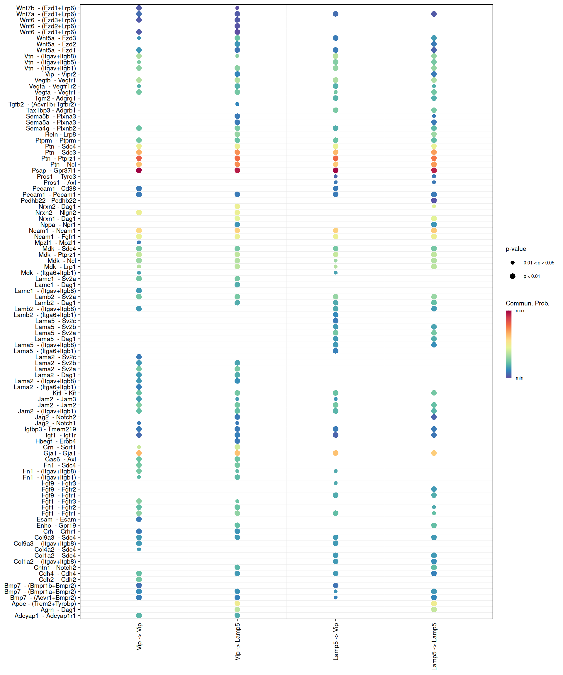
p1 + p2We can also visualise ligand-receptor interactions from one cell type to another with a bubble plot. Here, we look at interactions from Lamp5 to Vip and from Vip to Lamp5.
# Bubble plot of ligand-receptor interactions from Lamp5 to Vip and vice versa
netVisual_bubble(
  cell_chat,
  sources.use = c("Lamp5", "Vip"),
  targets.use = c("Lamp5", "Vip")
)
13.5 Pathway-level Visualisation
We can also focus on pathway-level communication, which we already computed above.
For this example, we look at two pathways of interest: COLLAGEN and LAMININ.
- Laminin is a key component of the extracellular matrix and plays an important role in cell adhesion, differentiation, migration and signalling. It is especially relevant in neural development and function, so it is a sensible pathway to inspect in brain tissue.
- Collagen is another major extracellular matrix component. It provides structural support and also contributes to cell adhesion and signalling.
We can use netAnalysis_contribution() to see how much each ligand-receptor pair contributes to those pathways.
# barplot of the contribution of each ligand-receptor interaction pair to the selected pathways
p1 <- netAnalysis_contribution(cell_chat, signaling = "COLLAGEN") +
  ggtitle("COLLAGEN pathway")

p2 <- netAnalysis_contribution(cell_chat, signaling = "LAMININ") +
  ggtitle("LAMININ pathway")

p1 +
  p2 +
  plot_annotation(title = "Contribution of ligand-receptor interaction pairs")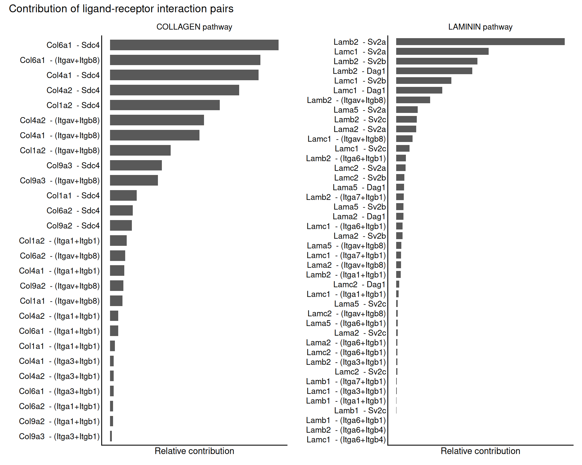
We can also compute centrality scores for selected pathways. These scores show how important each cell type is as a sender, receiver, mediator and influencer in the network.
# compute centrality scores for the selected pathways
cell_chat <- netAnalysis_computeCentrality(cell_chat)

# visualise the centrality scores for a selected pathway
netAnalysis_signalingRole_network(
  cell_chat,
  signaling = "LAMININ",
  width = 16,
  height = 8
)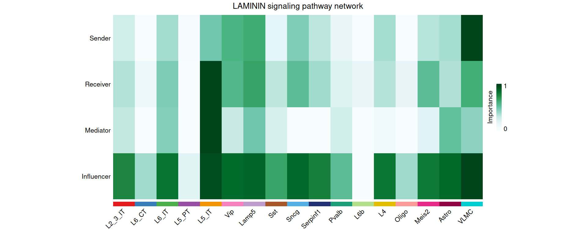
For the LAMININ pathway in this dataset, L5 IT is the most important receiver and VLMC is the most important sender.
We can get a broader view of each cell type’s role by comparing incoming and outgoing signalling strength across all pathways.
# All pathways
netAnalysis_signalingRole_scatter(cell_chat)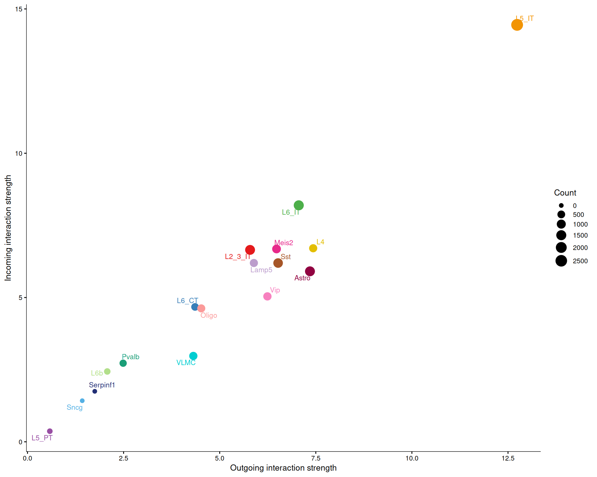
# Only the LAMININ pathway
netAnalysis_signalingRole_scatter(cell_chat, signaling = c("LAMININ"))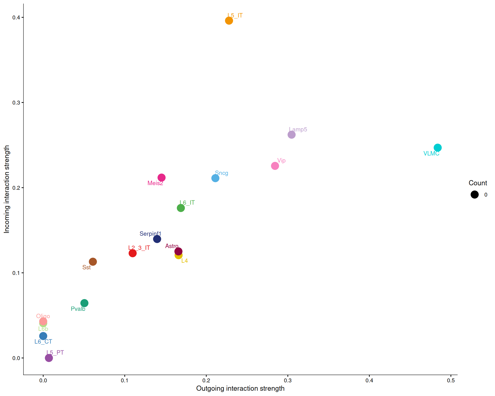
Across all pathways, there is usually a positive relationship between outgoing and incoming signalling strength. That makes sense, because cell types that send many signals also tend to receive many.
For the LAMININ pathway specifically, L5 IT is more active as a receiver than as a sender, while VLMC is more active as a sender than as a receiver. That pattern matches the centrality scores above.
13.6 Spatial Visualisation of Pathways
Finally, we can place a selected signalling pathway back into tissue context with netVisual_aggregate() and layout = "spatial".
netVisual_aggregate(
  cell_chat,
  signaling = "LAMININ",
  layout = "spatial",
  edge.width.max = 2,
  vertex.size.max = 1,
  alpha.image = 0.2,
  vertex.label.cex = 3.5
)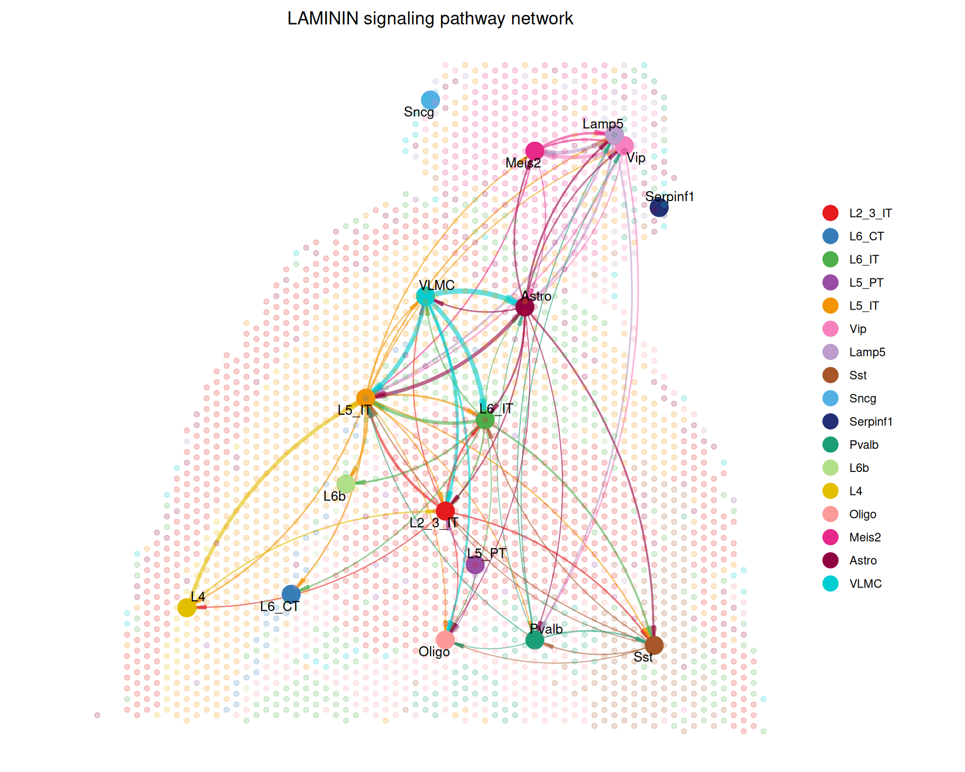
These spatial plots show the selected pathway in the context of the tissue. The nodes represent cell types, and the edges represent inferred interactions. Because the layout uses the spatial coordinates of the spots, you can see how communication is distributed across the tissue.
CellChat includes many other visualisation and exploration options. The package documentation is the best place to look for other visualisations that fit a specific dataset or research question.
13.7 Caveats and Limitations
Treat ligand-receptor networks inferred from single-cell or spatial transcriptomics as potential communication flows, not direct measurements of signalling activity. Most approaches, including CellChat, combine gene expression data with a curated database of known ligand-receptor interactions to identify relationships that are consistent with the observed data.
The main limitations of this approach are:
- mRNA is only a proxy for signalling protein abundance and activity. Expression of a ligand does not mean that the protein is produced and secreted, and expression of a receptor does not prove that the downstream pathway is active. Many signalling steps are regulated after transcription, for example by protein modification or receptor localisation, and transcriptomics does not capture those processes.
- Cell annotations strongly affect the result. Communication is usually inferred between cell populations, so incorrect annotations can hide real interactions. Over-clustering can also create artificial interactions between closely related cell states.
- The ligand-receptor database matters. Different databases contain different interaction sets and levels of curation, so the choice of database can change the interactions that are reported.
- Spatial proximity helps, but it does not prove communication. Nearby cells provide additional support for a possible interaction, but signalling can also occur over longer distances. Lower-resolution technologies may contain mixtures of cell types in a single spot, which makes it harder to assign interactions to individual cells.
- Use CCC results as hypotheses. Use the results to inform follow-up experiments, not definitive evidence of signalling. When possible, complement them with biological knowledge and experimental validation.
13.8 Summary
TipKey Points
- Cell-cell interactions are crucial for understanding tissue microenvironments and biological processes.
- Cell-cell communication analysis uses known ligand-receptor pairs to infer likely signalling relationships between cell populations.
- CCC results are hypotheses, not direct measurements of signalling.
CellChatuses a Seurat object, spatial conversion factors and spot coordinates to build a spatial communication model.- The ligand-receptor database controls which interactions
CellChatshould consider in its analysis. - CellChat visualisations show different views of the same inferred network.
- Circle plots summarise interaction counts and weights.
- Heatmaps highlight cell-type pairs with stronger connections.
- Bubble, pathway and spatial plots help interpret specific interactions.