# Load libraries
library(Seurat) # single-cell and spatial analysis toolkit
library(sparseMatrixStats)
library(paletteer) # colour palettes
library(ggplot2) # plotting
library(dplyr) # data manipulation
library(patchwork) # combining plots

# Load the Seurat object from the previous chapter
visium <- readRDS("precomputed/mouse_brain_banksy.rds")12 Deconvolution
TipLearning Objectives
- Explain why deconvolution is needed for lower-resolution spatial transcriptomics data and how spot resolution affects interpretation.
- Prepare compatible reference and query inputs for
spacexrfrom Seurat objects. - Run
create.RCTD()andrun.RCTD()with appropriatedoublet_modesettings for the biological and technical context. - Extract RCTD classifications and weights and add them to Seurat metadata for downstream analysis.
- Interpret and compare deconvolution outputs using spatial plots, thresholds, and heatmaps in the context of known tissue biology.
12.1 Setup
We continue working with the sagittal mouse brain dataset from previous chapters.
NoteClick to expand
Start by loading the required libraries and the Seurat object.
As a reminder, this object was created by:
- Importing the raw data using
Load10X_Spatial(), followed by QC and filtering to remove low-quality spots. - Data normalisation using
SCTransform(), which models technical variation and applies variance stabilisation. Stored in the “SCT” assay. - Applying dimensionality reduction using PCA, UMAP and t-SNE.
- Clustering the data using graph-based clustering. The clusters we use in this chapter were generated using the Leiden algorithm at a resolution of 0.8 and were set the the default cell identities (
Idents(visium)). - Identifying spatially variable features using Moran’s I and markvariogram methods.
- Running the BANKSY algorithm to identify spatial domains in the data, which were stored in the
banksy_clusterscolumn of the metadata.
12.2 Overview
Deconvolution estimates the cellular composition of mixed gene expression profiles. In spatial transcriptomics, this means estimating which cell types contribute to each pixel or spot. This is especially important for lower-resolution technologies, where each spot can capture multiple cells (for example Visium V1/V2 spots with 55 μm diameter). When those cells belong to different types, the measured expression is a mixture, which can affect downstream analyses such as clustering and tissue architecture analysis.
Several tools are available for spatial deconvolution, reviewed in Gaspard-Boulinc et al. 2022. Here we use Robust Cell Type Decomposition (RCTD) from Cable et al. 2022, which was one of the top-performing methods in that benchmark.
Briefly, RCTD requires:
- an annotated reference dataset (for example single-cell RNA-seq)
- a query spatial transcriptomics dataset to deconvolute
It then uses a probabilistic model to infer cell type mixtures in each spot.
RCTD is implemented in the spacexr package. We also load pheatmap for heatmap visualisations later in the chapter.
# Load necessary libraries
library(spacexr)
library(pheatmap)
Warning
spacexr package versions
Confusingly, there are two version of this package:
- The original package available from GitHub (dmcable/spacexr) has its own object structure and implements other methods not covered here.
- A re-implementation in Bioconductor using its standard
SpatialExperiment/SingleCellExperimentobjects. This package only implements the RCTD analysis of the original package.
While both provide similar functionality for RCTD analysis, the syntax is slightly different. We are using the original GitHub version here, so be aware that adaptations may be needed if you use the Bioconductor version instead.
12.3 Reference Dataset
The first step for deconvolution is choosing a suitable reference dataset. That choice depends on tissue, organism and data availability, and well-annotated references may be lacking for non-model organisms.
Here we use a preprocessed single-cell RNA-seq dataset from the Allen Brain Cell (ABC) Atlas. Cells are annotated hierarchically as class → subclass → cluster, from broad categories to specific cell populations.
- Class: broad categories such as glutamatergic neurons, GABAergic neurons, astrocytes, and oligodendrocytes.
- Subclass: groups within a class that share similar transcriptional profiles (for example Vip, Sst, and Lamp5 within GABAergic neurons).
- Cluster: the most specific level, often named with distinguishing marker genes (for example Vip Arhgap36 Hmcn1).
We start by loading the reference object and look at its structure. Because this is a precomputed object, we read it from RDS and run UpdateSeuratObject() for compatibility with current Seurat versions.
# Load the reference single-cell dataset
ref <- readRDS("precomputed/mouse_brain_reference_for_RCTD.rds")
ref <- UpdateSeuratObject(ref)

# Assays present in object
Assays(ref)
[1] "RNA" "SCT"This object includes an “RNA” assay with raw counts. It also includes an “SCT” assay containing sctransform-normalised data, set as the default assay.
Metadata includes the three annotation levels: class, subclass and cluster.
# Check the annotation levels in the reference dataset
ref[[]] |>
  select(class, subclass, cluster) |>
  head()
class subclass cluster
F1S4_160108_001_A01 GABAergic Vip Vip Arhgap36 Hmcn1
F1S4_160108_001_B01 GABAergic Lamp5 Lamp5 Lsp1
F1S4_160108_001_C01 GABAergic Lamp5 Lamp5 Lsp1
F1S4_160108_001_D01 GABAergic Vip Vip Crispld2 Htr2c
F1S4_160108_001_E01 GABAergic Lamp5 Lamp5 Plch2 Dock5
F1S4_160108_001_F01 GABAergic Sst Sst Tac1 Tacr3# Count how many of each annotation level we have
length(unique(ref$class))[1] 4length(unique(ref$subclass))[1] 22length(unique(ref$cluster))[1] 117We can visualise these annotations on a UMAP to see how they map onto cell populations.
Click to expand visualisation code
# Visualise UMAP and Spatial plots of the reference dataset with different annotation levels
umap_class <- DimPlot(
  ref,
  reduction = "umap",
  group.by = "class",
  label = TRUE
)
umap_subclass <- DimPlot(
  ref,
  reduction = "umap",
  group.by = "subclass",
  label = TRUE
)
umap_cluster <- DimPlot(
  ref,
  reduction = "umap",
  group.by = "cluster",
  label = FALSE
)

# Assemble the UMAPs together with common settings
(umap_class + umap_subclass + umap_cluster) &
  coord_equal() &
  theme_void() &
  theme(legend.position = "none")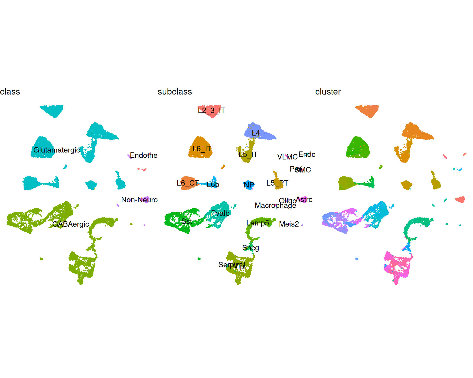
This can help us choose the annotation level for deconvolution. In this chapter we use the subclass level (22 categories), which gives a practical balance between granularity and interpretability.
Before running RCTD, check how many reference cells are available per subclass. If you use a different reference dataset, ensure each cell type has enough cells (at least 25) for a reliable estimation by RCTD.
# Count number of reference cells in each subclass
table(ref$subclass)
12.4 Preparing RCTD Data
RCTD requires both reference and query data in its own object formats.
12.4.1 Reference Object
The reference object needs:
- a count matrix
- cell type labels
- total UMI counts per cell
We extract these from the Seurat object and construct a Reference object.
# raw counts from the RNA assay
ref_counts <- ref[["RNA"]]$counts

# our cluster identities will be the subclass annotation
ref_cluster <- as.factor(ref$subclass)
names(ref_cluster) <- colnames(ref)

# the total number of UMIs for each cell
ref_umis <- ref$nCount_RNA
names(ref_umis) <- colnames(ref)

# Create the Reference object for RCTD
reference <- Reference(ref_counts, ref_cluster, ref_umis)

# Remove intermediate objects to free memory
rm(ref, ref_counts, ref_cluster, ref_umis)
12.4.2 Query Object
Similarly, we prepare the spatial dataset to deconvolute. RCTD needs:
- raw counts from the “Spatial” assay
- spot coordinates
- total UMI counts per spot
# raw counts
query_counts <- visium[["Spatial"]]$counts

# spot coordinates
query_coords <- GetTissueCoordinates(visium)[, c("x", "y")]

# total UMIs for each spot
query_umis <- colSums(query_counts)

# Construct the query object for RCTD
query <- SpatialRNA(query_coords, query_counts, query_umis)

# remove intermediate objects to free memory
rm(query_counts, query_coords, query_umis)
12.5 Running RCTD
With reference and query objects prepared, we can run deconvolution in two steps:
create.RCTD(): builds the RCTD object and prepares model inputs. This includes estimating cell type profiles from the reference, selecting informative genes (differentially expressed between classes), and estimating a normalisation factor to account for platform differences in the reference (e.g. single-cell versus single-nucleus).run.RCTD(): fits the model and estimates cell type proportions for each spot.
Run the first step to create the RCTD object:
# Create RCTD object on 8 cores
rctd <- create.RCTD(query, reference, max_cores = 8)

# Remove intermediate objects to free memory
rm(query, reference)
We set max_cores = 8 to reduce runtime, which can be substantial for larger datasets.
RCTD supports three deconvolution modes through doublet_mode:
"doublet": allows 1-2 cell types per spot. This is often suitable for higher-resolution spatial technologies."multi": similar to doublet mode but allows more than two cell types, up toMAX_MULTI_TYPESincreate.RCTD()(default 4)."full": places no explicit upper limit on the number of assigned cell types.
Constrained modes (“doublet” and “multi”) can reduce overfitting, where many very small proportions are assigned to each spot. The best choice depends on tissue complexity and spatial resolution of the technology.
We start with "doublet" mode and later compare results with "full" mode. RCTD is computationally demanding, so we provide a precomputed object. You can expand the code block below to see the command used.
Click for run.RCTD() command - takes a long time to run!
# This will run about ~12-15 minutes on 8 cores
rctd <- run.RCTD(rctd, doublet_mode = "doublet")
# Read precomputed rctd object in doublet mode
rctd <- readRDS("precomputed/mouse_brain_rctd_doublet.rds")We can now add the RCTD results to the Seurat object and for further analysis. Because we ran in doublet mode, we expect output describing major and secondary cell types per spot.
12.6 Extracting deconvolution results
The RCTD object stores results in several components. We extract the relevant parts into a data frame and then add them to the Seurat metadata.
We will extract:
- spot-level classification
- cell type weights (estimated proportions)
These values are in rctd@results:
# Main results data frame - retain only some columns of interest
doublet_results <- rctd@results$results_df |>
  select(spot_class, first_type, second_type)

# Add the associated with each type
doublet_results <- cbind(doublet_results, rctd@results$weights_doublet)

# Ensure column names are unique
names(doublet_results) <- c(
  "spot_class",
  "first_type",
  "second_type",
  "first_weight",
  "second_weight"
)

# Inspect the table
head(doublet_results)
spot_class first_type second_type first_weight
AAACAAGTATCTCCCA-1 doublet_certain Pvalb Oligo 0.7668344
AAACACCAATAACTGC-1 doublet_certain Astro Lamp5 0.5366842
AAACAGAGCGACTCCT-1 doublet_certain L5_IT Astro 0.8809316
AAACAGCTTTCAGAAG-1 doublet_certain Meis2 Astro 0.8719286
AAACAGGGTCTATATT-1 doublet_certain Meis2 Astro 0.8425738
AAACATTTCCCGGATT-1 doublet_certain Sst Astro 0.9213672
second_weight
AAACAAGTATCTCCCA-1 0.2331656
AAACACCAATAACTGC-1 0.4633158
AAACAGAGCGACTCCT-1 0.1190684
AAACAGCTTTCAGAAG-1 0.1280714
AAACAGGGTCTATATT-1 0.1574262
AAACATTTCCCGGATT-1 0.0786328Column meanings:
spot_class: spot classification ("singlet","doublet_uncertain","doublet_certain","reject").first_typeandsecond_type: the top two cell type assignments (using referencesubclasslabels).first_weightandsecond_weight: estimated proportions for those two assigned types.
Start by counting spots in each class:
# Count spot classes
doublet_results |>
  count(spot_class)
spot_class n
1 reject 7
2 doublet_certain 2515
3 doublet_uncertain 258We have no spots classified as “singlet”, which is expected given the spot size of Visium v1 and the complexity of the tissue. A high "doublet_certain" count indicates many spots are confidently modelled as mixtures of at least two types. "doublet_uncertain" and "reject" spots are useful to look at as well, because they can indicate ambiguous expression profiles or reference mismatches.
We can add these classifications to our Seurat metadata and visualise their spatial distribution:
# Add results back into visium object
visium <- AddMetaData(visium, metadata = doublet_results)

# Check where each spot is classified as a doublet
# We use a custom colour scheme to better distinguish the different classes
SpatialDimPlot(visium, group.by = "spot_class") +
  scale_fill_manual(
    values = c(
      "reject" = "red",
      "doublet_certain" = "steelblue",
      "doublet_uncertain" = "orange"
    )
  ) +
  ggtitle("Spot classification by RCTD")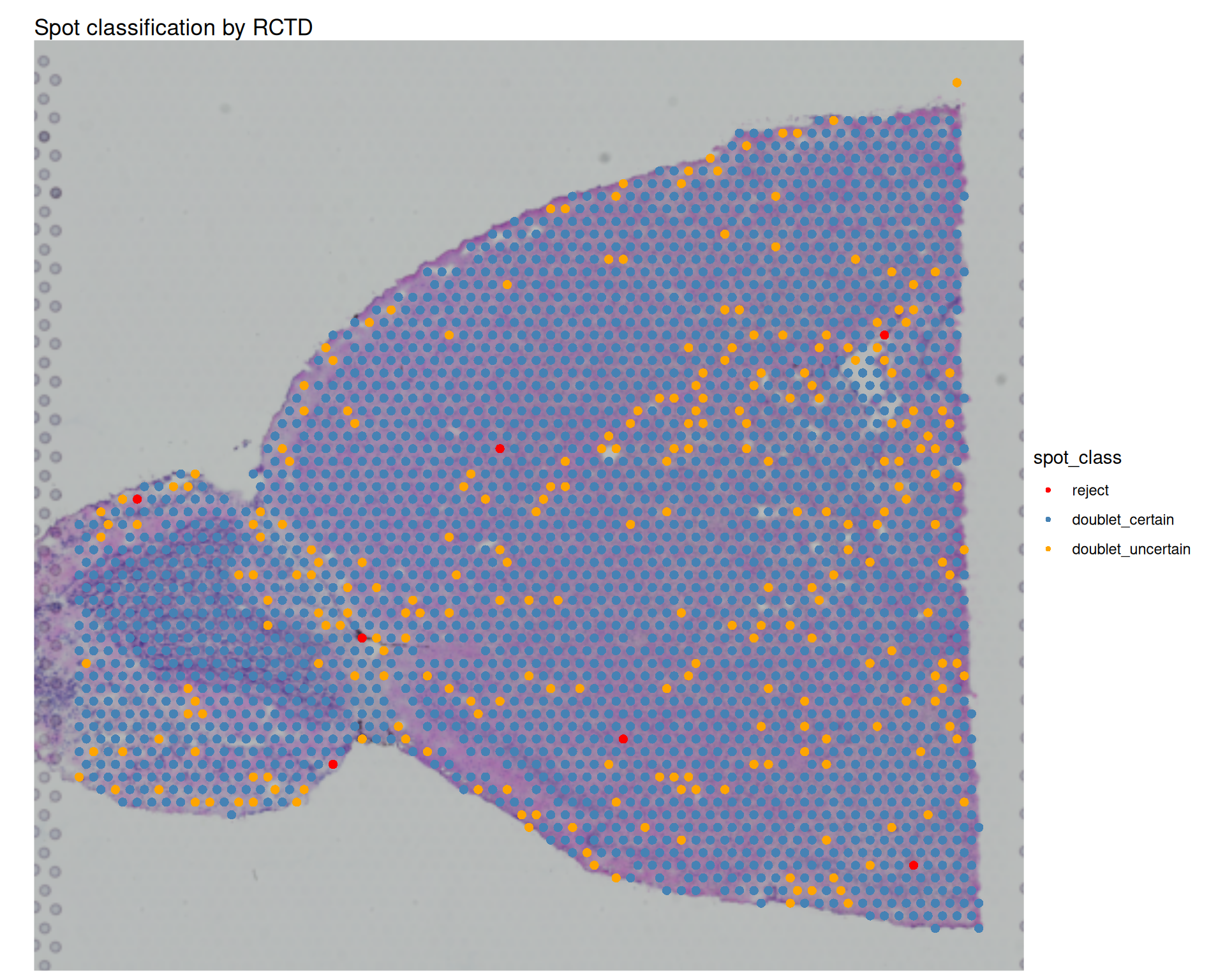
We can also compare RCTD type assignments with the Leiden clusters identified earlier:
Click for visualisation code
# Spatial plot for first type
first_type_plot <- SpatialDimPlot(
  visium,
  group.by = "first_type"
) +
  ggtitle("First cell type identified by RCTD")

# Spatial plot for second type
second_type_plot <- SpatialDimPlot(
  visium,
  group.by = "second_type"
) +
  ggtitle("Second cell type identified by RCTD")

# Leiden clusters
leiden_cluster_plot <- SpatialDimPlot(
  visium,
  group.by = "Leiden_08",
  label = TRUE,
  label.size = 4
) +
  theme(legend.position = "none") +
  ggtitle("Clusters (Leiden)")

# Assemble the plots together
(first_type_plot + second_type_plot) / leiden_cluster_plot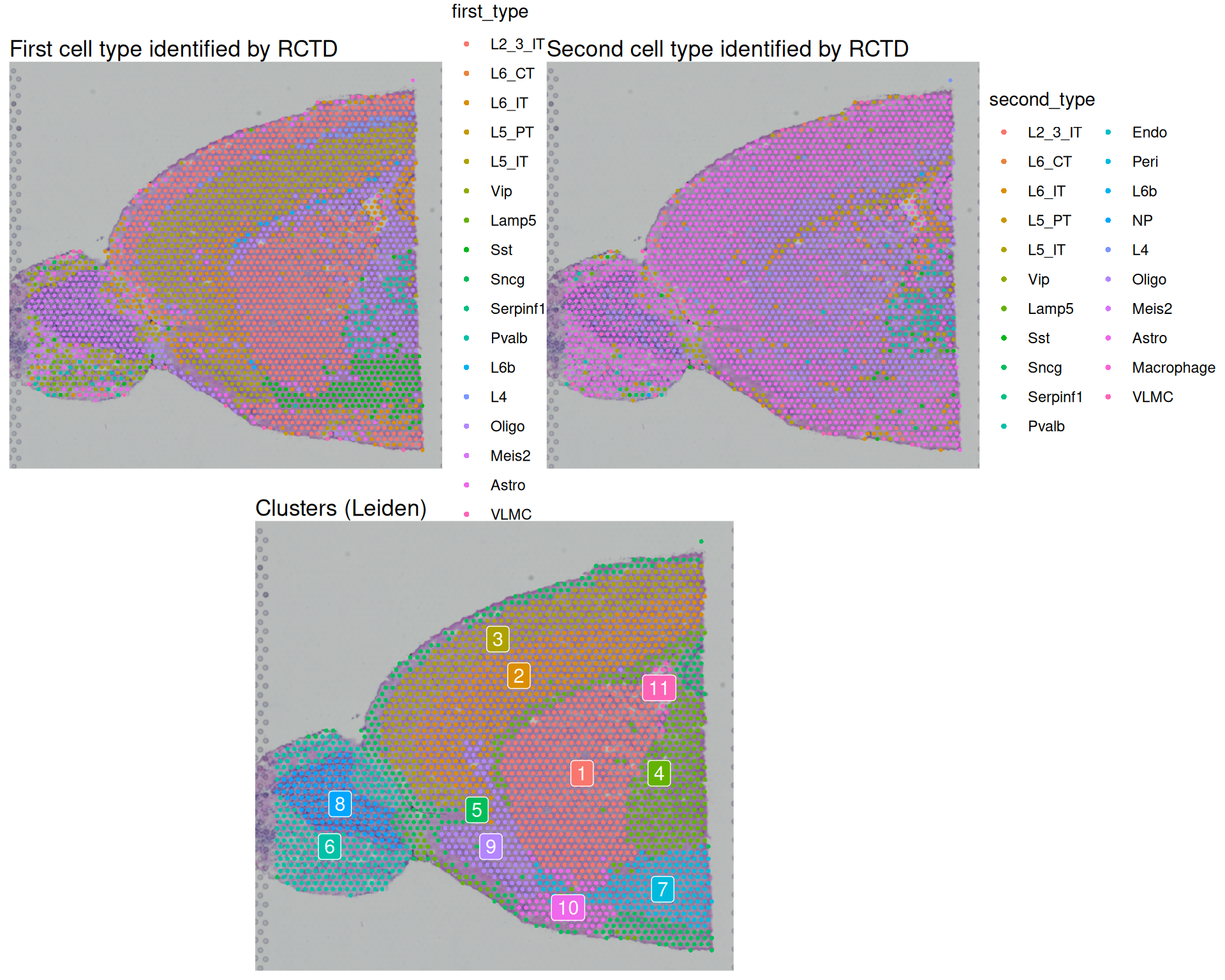
12.7 Full cell type analysis
So far we have focused on doublet mode, which reports the top one or two cell types per spot. This can be useful when spots are likely to contain only a small number of cell types.
For Visium v1, each 55 μm spot often contains multiple cells from several types. In this case, "full" mode may provide a more informative view of cell type composition in our spots.
Because this run is slow, we provide a precomputed file. The code below shows how it was generated.
Click for run.RCTD() command - takes a long time to run!
# Run RCTD in full mode
# Takes a long time to run! Read the precomputed object below instead
rctd_full <- run.RCTD(rctd, doublet_mode = "full")
# Read precomputed rctd object in doublet mode
rctd_full <- readRDS("precomputed/mouse_brain_rctd_full.rds")
NoteShould I always run RCTD in “full” mode?
Although it might sound like a good idea to always run the model in “full” mode, it is important to remember that the model may overfit the data, so it’s not a bad idea to restrict to doublets when working with high-resolution data.
In our case, as we are working with a low-resolution technology, it makes sense to attempt running the analysis in full mode.
12.7.1 Extract and visualise cell weights
In full mode, RCTD returns a weight matrix in rctd@results$weights. Rows correspond to spots, columns correspond to reference cell types, and each value is the estimated proportion of a cell type in a spot.
This can be used for two common tasks:
- broad exploration of all cell types
- analysis of specific types of interest
The next code block extracts and reshapes these weights for visualisation with ggplot2. We plot all subclasses to get a global view of composition patterns.
# Extract weights
rctd_weights <- rctd_full@results$weights

# Add coordinates
rctd_weights <- cbind(rctd_weights, GetTissueCoordinates(visium)[, c("x", "y")])

# Convert to tibble and pivot to long format
rctd_weights <- rctd_weights |>
  as_tibble(rownames = "spot_barcode") |>
  tidyr::pivot_longer(
    -c(spot_barcode, x, y),
    names_to = "subclass",
    values_to = "weight"
  )

# Visualise weights for each subclass
# Note we're capping the colour scale to 0.5 to better visualise differences
# We also use negative y values to match the orientation of the spatial plot
rctd_weights |>
  ggplot(aes(x, -y, colour = weight)) +
  geom_point(size = 0.1) +
  facet_wrap(~subclass) +
  theme_void() +
  scale_colour_viridis_c(limits = c(0, 0.5))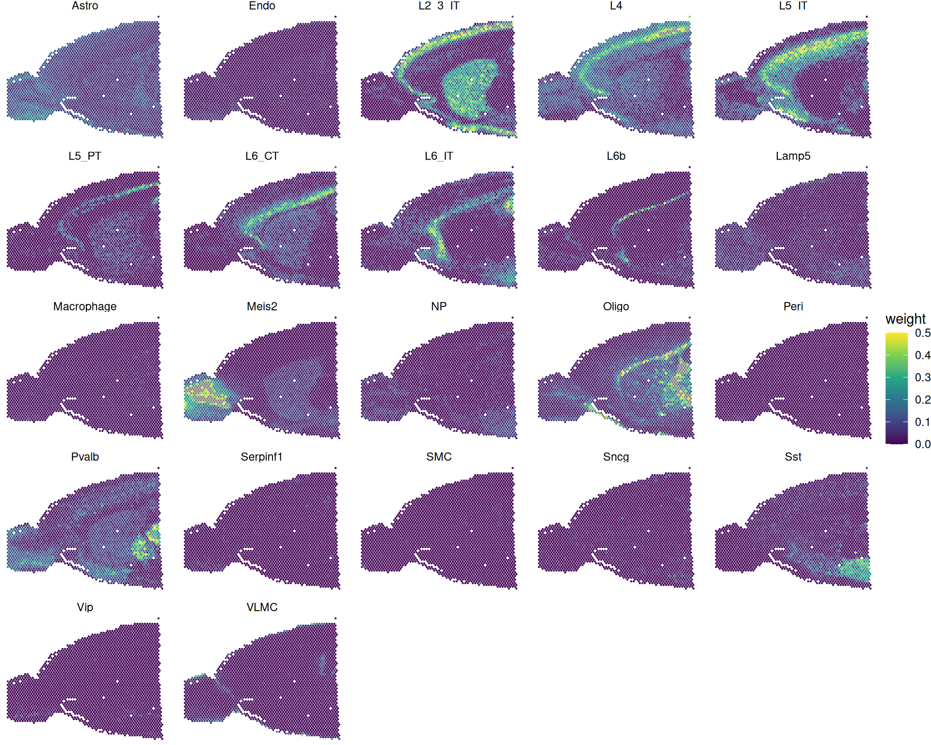
As always, you should interpret these results grounded in biological knowledge of the tissue and cell types you are looking at. You can focus on whether high-weight regions align with expected anatomical locations. Unexpected patterns can reflect genuine biology, reference limitations, or model overfitting.
For example, consider cell type “L2_3_IT” (layer 2/3 intratelencephalic neurons; see ABC Atlas entry):
Code
# Highlight a particular cell type
SpatialPlot(
  visium,
  cells.highlight = WhichCells(visium, expression = first_type == "L2_3_IT")
)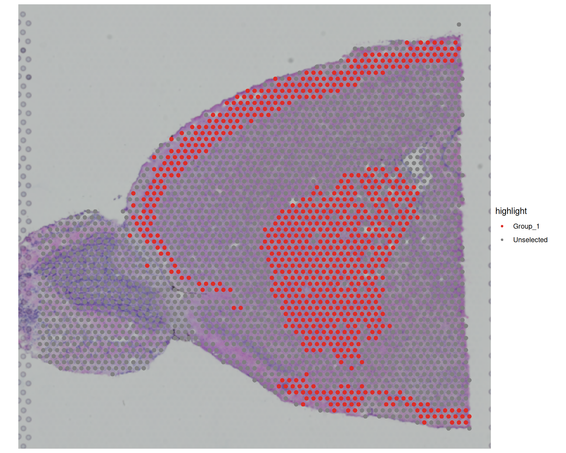
These spots appear in superficial cortical layers, which is biologically plausible. However, we also see a strong signal in inner tissues, which may be less expected.
Here are a couple of reasons why you might see a signal in less expected regions:
- Model overfitting assigns low-confidence contributions, when in fact that cell type is absent.
- The reference lacks true matching cell states, so the model assigns the closest available type.
For this reason, treat deconvolution as one source of evidence and cross-check with marker genes, spatial context and tissue knowledge.
12.7.2 Add cell weights to Seurat
As with doublet-mode results, we can add full-mode weights to Seurat metadata:
# Add cell type weights to metadata
visium <- AddMetaData(visium, rctd_full@results$weights)

# Check this has been added as new columns to metadata
colnames(visium[[]])
[1] "orig.ident" "nCount_Spatial" "nFeature_Spatial"
[4] "percentMt_Spatial" "nCountFiltered" "percentMtFiltered"
[7] "nFeatureFiltered" "combinedFiltered" "nCount_SCT"
[10] "nFeature_SCT" "scranSizeFactors" "SCT_snn_res.0.8"
[13] "seurat_clusters" "Louvain_05" "Leiden_05"
[16] "Louvain_08" "Leiden_08" "banksy_cluster"
[19] "spot_class" "first_type" "second_type"
[22] "first_weight" "second_weight" "L2_3_IT"
[25] "L6_CT" "L6_IT" "L5_PT"
[28] "L5_IT" "Vip" "Lamp5"
[31] "Sst" "Sncg" "Serpinf1"
[34] "Pvalb" "Endo" "Peri"
[37] "L6b" "NP" "L4"
[40] "Oligo" "Meis2" "Astro"
[43] "Macrophage" "VLMC" "SMC" You now have one metadata column per cell type, containing RCTD weight estimates. These columns can be used directly in spatial plots or dimensionality-reduction plots.
12.7.3 Identify most abundant type
We can also assign each spot its most abundant inferred cell type. Using the long-format weights table, we select the highest-weight subclass per spot and add it back to metadata.
max_cell_type <- rctd_weights |>
  # for each barcode
  group_by(spot_barcode) |>
  # get the cell type with the highest weight
  slice_max(weight) |>
  ungroup()

# add to metadata - make sure to match the order of the barcodes
visium$rctd_max_type <- max_cell_type$subclass[match(
  colnames(visium),
  max_cell_type$spot_barcode
)]
visium$rctd_max_weight <- max_cell_type$weight[match(
  colnames(visium),
  max_cell_type$spot_barcode
)]

# Visualise the most abundant cell type in each spot
SpatialDimPlot(visium, group.by = "rctd_max_type") +
  ggtitle("Most abundant cell type in each spot")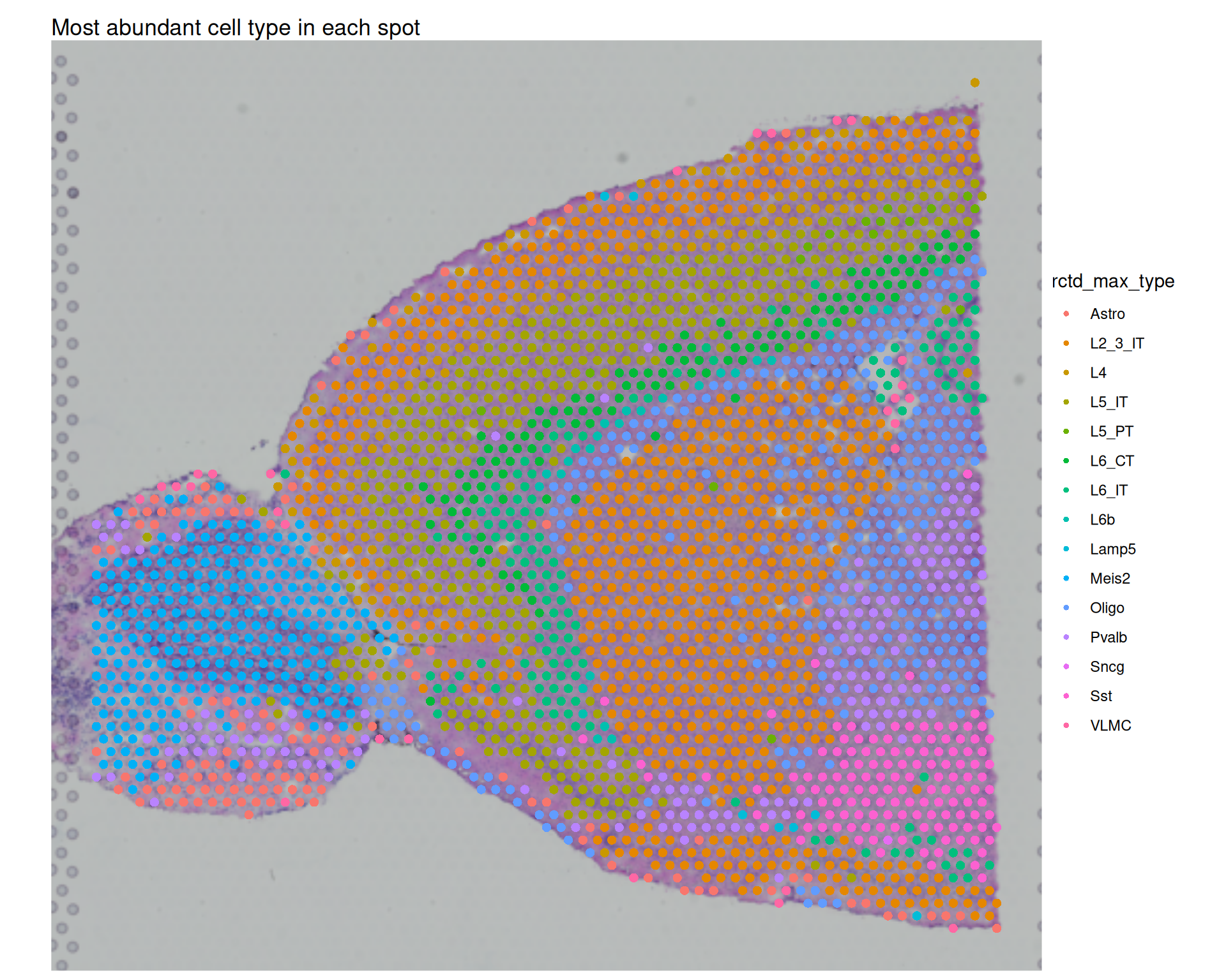
You can also apply a confidence threshold, for example only assigning a label if the maximum weight is above 0.5:
# add metadata column indicating whether the max weight is greater than 0.5
visium$rctd_max_type_gt_05 <- ifelse(
  visium$rctd_max_weight > 0.5,
  visium$rctd_max_type,
  NA
)

# Visualise the most abundant cell type with weight > 0.5
SpatialDimPlot(visium, group.by = "rctd_max_type_gt_05") +
  ggtitle("Most abundant cell type in each spot (weight > 0.5)")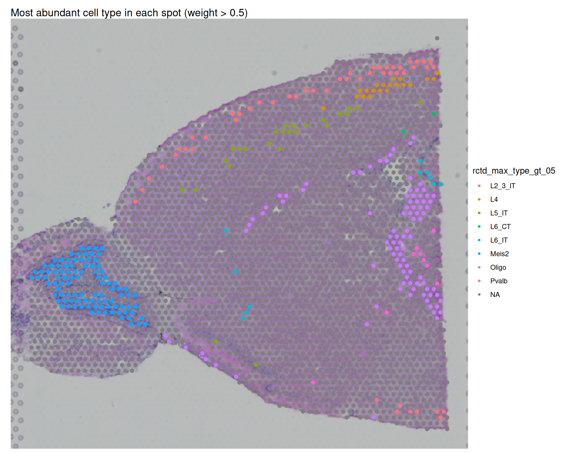
If very few spots pass this threshold, that suggests most spots are mixed, which is expected for Visium v1. It can also indicate that full mode is distributing small weights across many candidate types.
You can explore these thresholds to explore the deconvolution results in different ways, and to identify the most likely cell type in each spot based on the weights assigned by RCTD.
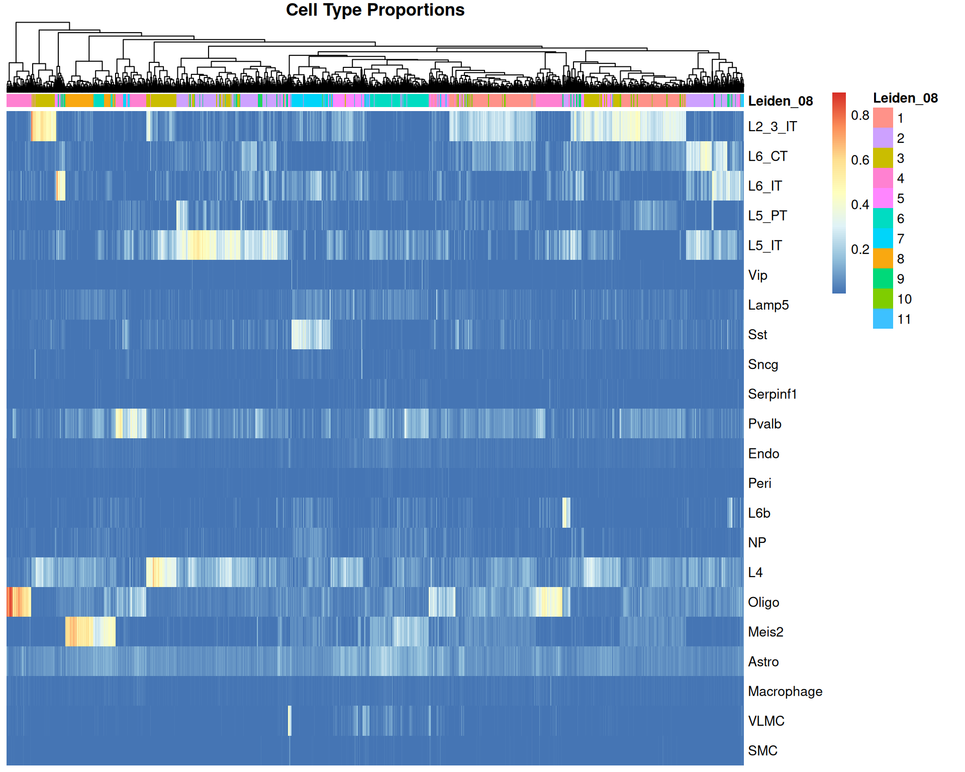
12.7.4 Weight Heatmaps
We can also inspect cell type proportions as a heatmap. One useful strategy is ordering spots by previous clustering labels. Here we order spots by the Leiden_08 metadata column from the previous chapter.
# prepare heatmap matrix from weights matrix
# order the rows (spots) based on Leiden clusters
heatmap_data <- rctd_full@results$weights[order(visium$Leiden_08), ]

# Transpose the matrix for easier heatmap interpreation (cell types as rows, spots as columns)
heatmap_data <- t(heatmap_data)

# Visualise as heatmap adding leiden cluster annotation
pheatmap(
  heatmap_data,
  cluster_rows = FALSE,
  cluster_cols = FALSE,
  show_colnames = FALSE,
  annotation_col = data.frame(Leiden_08 = sort(visium$Leiden_08)),
  main = "Cell Type Proportions"
)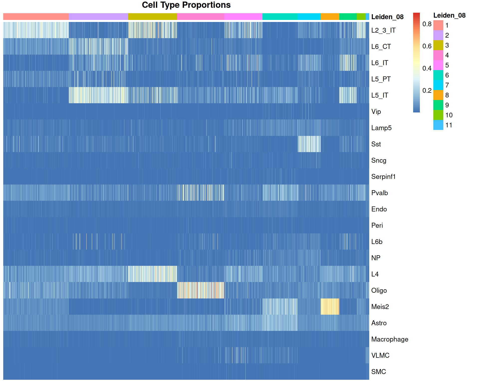
We can see some correlation between the Leiden clusters and the cell type proportions, which is expected as both are based on gene expression profiles. But this is not a perfect alignment, we can see many scattered spots with high proportions of certain cell types that do not correlate with these clusters. We might expect this result as each spot likely contains multiple cell types, and the clustering is based on the overall gene expression profile of the spot, which can be confused by the presence of multiple cell types.
Alternatively, you can cluster the heatmap columns to group spots by composition similarity:
# Heatmap with clustered spots
pheatmap(
  heatmap_data,
  cluster_rows = FALSE,
  cluster_cols = TRUE,
  show_colnames = FALSE,
  annotation_col = data.frame(Leiden_08 = sort(visium$Leiden_08)),
  main = "Cell Type Proportions"
)
This view shows spot groups that do not perfectly match expression-defined clusters.
For example, there is a small cluster of spots with high “L6b” proportions:
Code
# Spatial plot for L6b weight
spatial_l6b <- SpatialFeaturePlot(visium, features = "L6b") +
  ggtitle("L6b cell type")

# UMAP with these cells highlighted
umap_l6b <- DimPlot(
  visium,
  reduction = "umap",
  cells.highlight = WhichCells(visium, expression = rctd_max_type == "L6b")
) +
  theme(legend.position = "none") +
  coord_equal() +
  theme_void()

spatial_l6b + umap_l6b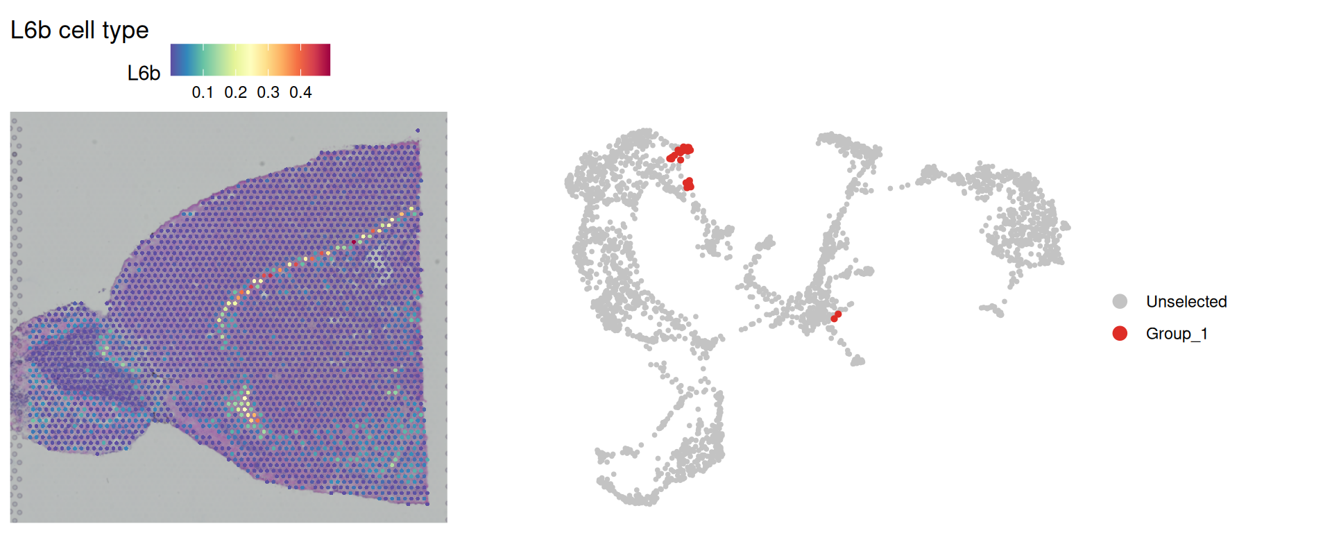
These spots form a narrow spatial band, often close to a single line of spots. That pattern is consistent with layer 6b neurons occupying a thin cortical layer.
This example also shows why analysis resolution matters. In the previous spatial clustering chapter, BANKSY used k_geom = 18, averaging spatial features across 18 neighbouring spots (two rings of spots around each spot). For very narrow structures, this averaging can dilute local signals and make small sub-domains harder to identify.
This again highlights the importance of biological knowledge of your tissue and considering the resolution of the technology used.
12.8 Exporting Seurat Object
Optionally, save the Seurat object with deconvolution results for later use:
# Save Seurat object
saveRDS(visium, "results/mouse_brain_visium_deconvolution.rds")
12.9 Summary
TipKey Points
Deconvolution helps identify cell type mixtures in spatial spots where multiple cells contribute to one expression profile.
- Spot size and tissue complexity determine how strongly mixed each spot is likely to be.
- Mode choice (
doubletversusfull) depends on the expected number of contributing cell types.
spacexrrequires reference and query objects for model fitting.Reference()uses raw counts, cell labels, and per-cell UMIs from the single-cell reference.SpatialRNA()uses spot coordinates, raw counts, and per-spot UMIs from the spatial dataset.
RCTD runs in two stages: object construction with
create.RCTD()and deconvolution withrun.RCTD().Doublet-mode outputs gives spot classes and top cell type assignments that can be integrated into Seurat metadata.
spot_classdistinguishes confident doublets, uncertain doublets, and rejected spots.first_type/second_typeand their weights provide the two inferred cell types and their frequencies.
Full-mode weights can be used for a more exhaustive analysis of cell types.
- Heatmaps and spatial plots can be used to compare composition patterns with previous clustering results.
- Results should always be compared to known tissue biology and interpreted with caution.