# Load libraries
library(Seurat) # single-cell and spatial analysis toolkit
library(sparseMatrixStats)
library(paletteer) # colour palettes
library(ggplot2) # plotting
library(dplyr) # data manipulation
library(patchwork) # combining plots

# Load the Seurat object from the previous chapter
visium <- readRDS("precomputed/mouse_brain_clustering.rds")10 Spatially Variable Features
TipLearning Objectives
- Distinguish between highly variable genes (HVGs) and spatially variable genes (SVGs) in spatial transcriptomics data.
- Identify spatially variable features and visualise their spatial expression patterns.
- Apply Moran’s I and markvariogram methods to rank features by spatial variability.
- Compare Moran’s I and markvariogram results for spatially variable features.
- Explain how spatially variable features can inform biological interpretation.
10.1 Setup
We continue working with the sagittal mouse brain dataset from previous chapters.
NoteClick to expand
Start by loading the required libraries and the Seurat object.
As a reminder, this object was created by:
- Importing the raw data using
Load10X_Spatial(), followed by QC and filtering to remove low-quality spots. - Data normalisation using
SCTransform(), which models technical variation and applies variance stabilisation. Stored in the “SCT” assay. - Applying dimensionality reduction using PCA, UMAP and t-SNE.
- Clustering the data using graph-based clustering. The clusters we use in this chapter were generated using the Leiden algorithm at a resolution of 0.8 and were set the the default cell identities (
Idents(visium)).
10.2 Overview
In the dimensionality reduction chapter, we selected highly variable genes (HVGs) using a non-spatial approach. That approach treats spots as independent observations and does not use their positions in the tissue.
Here, we use spatially aware feature selection to identify spatially variable genes (SVGs), i.e. genes whose expression changes across the tissue.
SVGs are useful for at least two reasons:
- They complement cluster marker gene analysis by highlighting genes associated with spatial tissue structure and local biological processes.
- They can be used as input features for PCA, which can then influence downstream analyses such as UMAP, t-SNE and graph-based clustering.
Many SVG methods adapt ideas from spatial statistics. Two methods used in Seurat are:
- Moran’s I: measures whether nearby spots have similar expression values.
- Moran’s I ranges from -1 to 1.
- Negative values suggest dispersed expression patterns (for example, expression in separated regions).
- Positive values suggest local clustering (for example, higher expression concentrated in one tissue area).
- Values near zero correspond to no consistent spatial structure, i.e. a random spatial pattern.
- Markvariogram: measures how expression differences between spot pairs change with distance.
- A gene is spatially variable when nearby and distant spot pairs show different variance patterns.
- This can capture complex structures such as gradients or periodic patterns.
10.3 Identifying SVGs
Seurat provides FindSpatiallyVariableFeatures() to identify SVGs. The function supports Moran’s I and markvariogram (the default method).
Here, we use Moran’s I and keep the top 2000 spatially variable features:
# Identify spatially variable features using the "moransi" method
visium <- FindSpatiallyVariableFeatures(
  visium,
  assay = "SCT",
  selection.method = "moransi",
  nfeatures = 2000
)

# View the top spatially variable features
SpatiallyVariableFeatures(visium)[1:10]
[1] "Gng4" "Calb2" "Ttr" "Fabp7" "Doc2g" "S100a5" "Pcbp3"
[8] "Nrgn" "Ppp1r1b" "Gpr88" SpatiallyVariableFeatures() returns a vector of the feature names, ranked by spatial variability score. We can plot some of these in a spatial plot and compare their pattern with our previous cluster assignments to see how they correlate.
# Visualise the top nine spatially variable features for a 3x3 grid
SpatialFeaturePlot(
  visium,
  features = SpatiallyVariableFeatures(visium)[1:9],
  ncol = 3
)
# Visualise the Leiden clusters (default Idents)
SpatialDimPlot(
  visium,
  label = TRUE,
  label.size = 3
) +
  theme(legend.position = "none")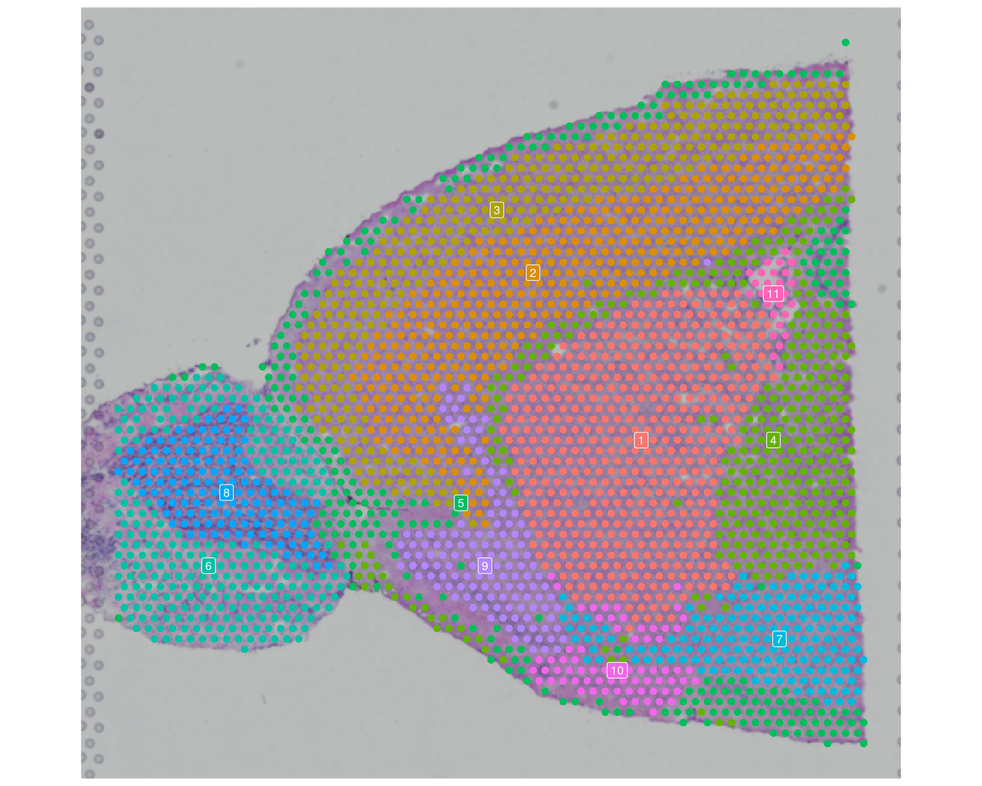
When you interpret these plots, look for repeated boundaries or gradients across multiple SVGs. Patterns that occur in several genes may indicate robust tissue structure, rather than a more spurious result from a single feature.
You will often see partial overlap between SVG patterns and cluster boundaries. That is expected: Leiden clustering here is graph-based and does not explicitly model spatial coordinates, but it can still recover biologically spatially organised cell populations.
We come back to spatially aware clustering in 08-TissueArchitecture.qmd, where we compare those clusters and their marker genes with the SVGs identified here.
NoteAccessing full Moran’s I results
The FindSpatiallyVariableFeatures() function adds the Moran’s I results to the feature metadata of the assay used (SCT). You can inspect that table to explore the full results, for example by filtering SVGs on Moran’s I values or plotting the score distribution.
To access the feature metadata, use [[]] on the relevant assay object:
# View the feature metadata for the "SCT" assay
head(visium[["SCT"]][[]])
MoransI_observed MoransI_p.value moransi.spatially.variable
Xkr4 NA NA NA
Gm19938 NA NA NA
Sox17 NA NA NA
Mrpl15 NA NA NA
Lypla1 NA NA NA
Tcea1 NA NA NA
moransi.spatially.variable.rank
Xkr4 NA
Gm19938 NA
Sox17 NA
Mrpl15 NA
Lypla1 NA
Tcea1 NAThis returns a standard data frame, so you can use dplyr and ggplot2 to manipulate and visualise it.
# Get the feature metadata for the "SCT" assay
feature_metadata <- visium[["SCT"]][[]]

# Histogram of Moran's I statistic
feature_metadata |>
  # remove NA values, which retains only significant genes
  filter(moransi.spatially.variable) |>
  ggplot(aes(MoransI_observed)) +
  geom_histogram()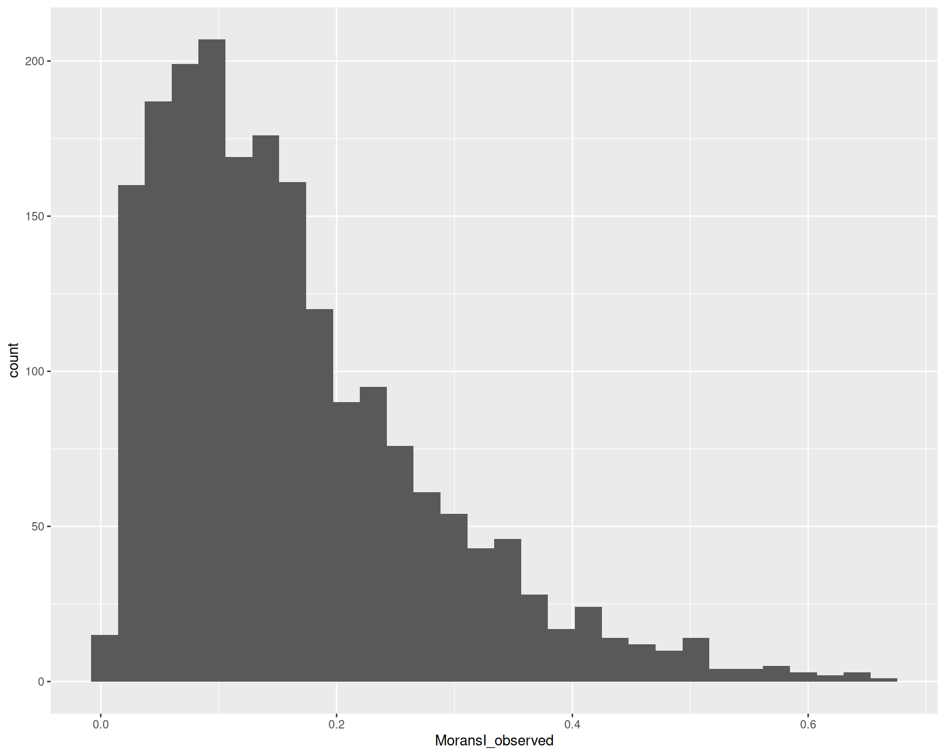
10.4 Markvariogram method
We can compare the SVGs identified with Moran’s I to those identified with markvariogram. To do that, run FindSpatiallyVariableFeatures() again with selection.method = "markvariogram".
The markvariogram method is slower than Moran’s I, so this chapter uses a precomputed object to save time. You can expand the code block below to see the code used.
Run FindSpatiallyVariableFeatures with markvariogram - takes a long time, read precomputed object instead
# Identify spatially variable features using the "markvariogram" method
# Takes a long time to run! Read the precomputed object below instead
visium <- FindSpatiallyVariableFeatures(
  visium,
  assay = "SCT",
  selection.method = "markvariogram",
  nfeatures = 2000
)
# Load precomputed markvariogram results
visium <- readRDS("precomputed/mouse_brain_svgs.rds")After running the function again, SpatiallyVariableFeatures() returns the top 2000 SVGs identified with markvariogram instead of Moran’s I.
# View the top spatially variable features identified with markvariogram
SpatiallyVariableFeatures(visium)[1:10]
[1] "Gng4" "Calb2" "Ttr" "Fabp7" "Doc2g" "S100a5" "Pcbp3"
[8] "Nrgn" "Ppp1r1b" "Gpr88" You may notice that the top SVGs identified with markvariogram are similar to those identified with Moran’s I, although their rankings may differ. We can check this more systematically by looking at the feature metadata, which contains results for both methods.
# Extract the feature (gene) metadata
feature_metadata <- visium[["SCT"]][[]]

# Look at the top columns of significant SVGs from both methods
feature_metadata |>
  filter(moransi.spatially.variable | markvariogram.spatially.variable) |>
  head()
MoransI_observed MoransI_p.value moransi.spatially.variable
Rgs20 0.09216726 0.0009756098 TRUE
Oprk1 0.13455745 0.0009756098 TRUE
Vxn 0.48917162 0.0009756098 TRUE
Sgk3 0.04343199 0.0009756098 TRUE
Sulf1 0.13691378 0.0009756098 TRUE
Kcnb2 0.19871834 0.0009756098 TRUE
moransi.spatially.variable.rank r.metric.5
Rgs20 1351 0.8683005
Oprk1 1020 0.7997586
Vxn 38 0.2616358
Sgk3 1780 0.9399345
Sulf1 1003 0.7065353
Kcnb2 601 0.7219798
markvariogram.spatially.variable markvariogram.spatially.variable.rank
Rgs20 TRUE 1553
Oprk1 TRUE 1162
Vxn TRUE 34
Sgk3 TRUE 1918
Sulf1 TRUE 751
Kcnb2 TRUE 808# get the moran's I and markvariogram gene ids
moransi_genes <- feature_metadata |>
filter(moransi.spatially.variable) |>
rownames()
markvariogram_genes <- feature_metadata |>
filter(markvariogram.spatially.variable) |>
rownames()
# quick Venn diagram of the overlap between the two methods
gplots::venn(list(MoransI = moransi_genes, Markvariogram = markvariogram_genes))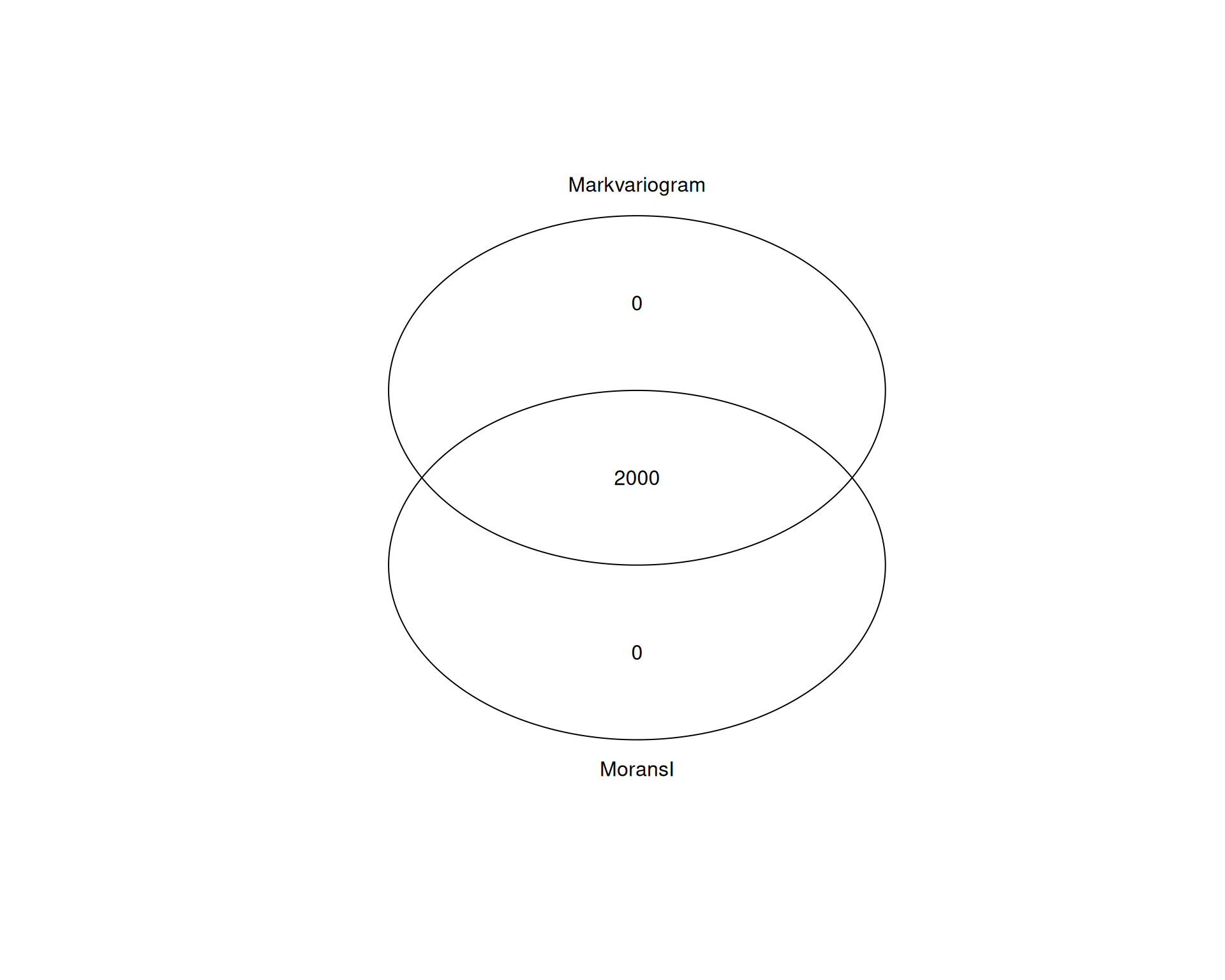
All 2000 genes are shared between both methods. That is not surprising, because both methods aim to capture spatial variability, even though they use different statistical approaches.
In this dataset, either method gives the same set of SVGs to work with. However, it is still worth comparing methods in other tissues, where more complex spatial patterns may be captured better by one approach than the other.
TipBiological interpretation of spatially variable genes
Spatially variable genes can highlight biological structure, including tissue organisation, cell-cell communication and local responses to environmental cues. After identifying SVGs, you can test their functional relevance with pathway enrichment analysis or gene ontology analysis, as in earlier cluster marker gene analysis.
10.5 Summary
TipKey Points
- Seurat can identify spatially variable features with
FindSpatiallyVariableFeatures().- Moran’s I and markvariogram both score features for spatial variation.
SpatiallyVariableFeatures()returns the top-ranked features from the most recent method used.
- Spatial feature plots help you compare SVG patterns with cluster structure.
- Repeated boundaries or gradients across multiple genes suggest robust spatial structure.
- Partial overlap with clusters is expected, because the clusters here are graph-based rather than spatially aware.
- The active assay stores feature metadata for the Moran’s I and markvariogram results.
- Use
visium[["SCT"]][[]]to access the full feature metadata table. - You can filter or plot that table to explore the distribution of the spatial statistics scores.
- Use
- Spatially variable features can suggest biological roles worth following up.
- They may reflect tissue organisation, cell-cell communication or responses to local cues.
- Pathway enrichment and gene ontology analysis can help interpret them.