5 Preprocessing Spatial Transcriptomics Data

Learning Objectives

Perform quality control on spatial transcriptomics data
Identify and remove low-quality cells
Normalise and scale spatial transcriptomics data

5.1 Introduction

Preprocessing spatial transcriptomics data is a crucial step in ensuring the quality and reliability of the analysis. Today we will be working on the Visium mouse dataset we loaded from raw data and saved as a Seurat object in the previous session. The preprocessing steps include scaling, normalization, quality control, and filtering of low-quality cells. We will keep working with the Seurat object visium that we created in the previous chapter.

5.2 Quality Control

Quality control (QC) is crucial to ensure the reliability of the data. In Seurat, you can perform QC by calculating metrics such as the number of detected genes, percentage of mitochondrial genes, and total counts per cell. You can then filter out low-quality spots based on these metrics.

# Calculate QC metrics
visium[["percent.mt"]] <- PercentageFeatureSet(visium, pattern = "^mt-")
visium[["nCount_Spatial"]] <- Matrix::colSums(visium@assays$Spatial)

5.3 Identifying and Removing Low-Quality Cells

After calculating the QC metrics, you can visualize them using scatter plots or histograms to identify low-quality cells. You can then remove these cells from the dataset.

# Visualize QC metrics
VlnPlot(visium, features = c("nCount_Spatial", "percent.mt"), ncol = 2)
# Remove low-quality cells and check the difference in metrics
visium <- subset(visium, subset = nCount_Spatial > 1000 & percent.mt < 25)
VlnPlot(visium, features = c("nCount_Spatial", "percent.mt"), ncol = 2)

We are removing cells with low total counts (less than 1000) and high mitochondrial percentage (greater than 25%). You can adjust these thresholds based on your specific dataset and analysis requirements. Sometimes it is also useful to look at the number of detected genes per cell (nFeature_Spatial) as an additional QC metric.

# Visualize number of detected genes per cell
VlnPlot(visium, features = c("nFeature_Spatial"), ncol = 1)

This can help identify cells with very low gene detection, which may indicate low-quality cells. Cells with unusually high numbers of detected genes may also be indicative of doublets or multiplets, which can be filtered out as needed. The expected range for nFeature_Spatial will depend on the specific dataset, experimental conditions and especially the species and technology used.

5.4 Scaling and Normalization

Scaling and normalization are essential steps in preprocessing spatial transcriptomics data to ensure that the data is comparable across different cells and conditions. In Seurat, this can be done using the SCTransform function, which performs normalization and variance stabilization. If you are working with a large dataset, consider using the vars.to.regress parameter to regress out unwanted sources of variation, such as the percentage of mitochondrial genes. We are also reducing the number of cells used for normalization to speed up the process and reduce memory requirements, but you can adjust this based on your dataset size and computational resources. As this step still requires a lot of memory, it is recommended to run it on a machine with sufficient RAM.

# Perform SCTransform normalization
visium <- SCTransform(visium, assay = "Spatial", verbose = FALSE, ncells = 5000, vars.to.regress = "percent.mt")

We are using SCTransform here, but Seurat also includes the NormalizeData function that performs simple log-normalisation. For spatial data, SCTransform is generally preferred due to its ability to handle technical variability more effectively. Additionally, when including the regression of mitochondrial percentage, SCTransform tends to run more efficiently than NormalizeData with ScaleData, thus saving both time and memory.

Investigating Normalization Methods and Mitochondrial Regression

If you would like to compare the results of SCTransform with NormalizeData, you can do so by following these steps. They include basic clustering and UMAP visualization to compare the outcomes of both normalization methods, with and without regressing out mitochondrial percentage. We will cover clustering and UMAP visualization in more detail in later sections, for now we will just use them to better visualize the differences in normalization methods.

#SCTransform with mitochondrial regression
visiumSCTmt <- SCTransform(visium, assay = "Spatial", verbose = TRUE,
                      ncells = 2000, conserve.memory = TRUE,
                      variable.features.n = 2000, vst.flavor="v2",
                      vars.to.regress = "percent.mt")
visiumSCTmt <- RunPCA(visiumSCTmt, assay = "SCT", verbose = FALSE)
visiumSCTmt <- RunUMAP(visiumSCTmt, assay = "SCT", reduction.name = "umap", dims = 1:30, reduction.key = "UMAP")
visiumSCTmt <- FindNeighbors(visiumSCTmt, assay = "SCT", reduction = "pca", dims = 1:30)
visiumSCTmt <- FindClusters(visiumSCTmt, resolution = 0.5)

#SCTransform without mitochondrial regression
visiumSCT <- SCTransform(visium, assay = "Spatial", verbose = TRUE,
                           ncells = 2000, conserve.memory = TRUE,
                           variable.features.n = 2000, vst.flavor="v2")
visiumSCT <- RunPCA(visiumSCT, assay = "SCT", verbose = FALSE)

visiumSCT <- RunUMAP(visiumSCT, assay = "SCT", reduction.name = "umap", dims = 1:30, reduction.key = "UMAP")
visiumSCT <- FindNeighbors(visiumSCT, assay = "SCT", reduction = "pca", dims = 1:30)
visiumSCT <- FindClusters(visiumSCT, resolution = 0.5)


#Log-normalisation with mitochondrial regression
visiumScaleMT <- NormalizeData(visium, assay = "Spatial", normalization.method = "LogNormalize", scale.factor = 10000)
visiumScaleMT <- ScaleData(visiumScaleMT, assay = "Spatial", vars.to.regress = "percent.mt")
visiumScaleMT <- FindVariableFeatures(visiumScaleMT)
visiumScaleMT <- RunPCA(visiumScaleMT, assay = "Spatial", verbose = FALSE)
visiumScaleMT <- RunUMAP(visiumScaleMT, assay = "Spatial", reduction.name = "umap",  dims = 1:30, reduction.key = "UMAP")
visiumScaleMT <- FindNeighbors(visiumScaleMT, assay = "Spatial", reduction = "pca", dims = 1:30)
visiumScaleMT <- FindClusters(visiumScaleMT, resolution = 0.5)

#Log-normalisation without mitochondrial regression
visiumScale <- NormalizeData(visium, assay = "Spatial", normalization.method = "LogNormalize", scale.factor = 10000)
visiumScale <- ScaleData(visiumScale, assay = "Spatial")
visiumScale <- FindVariableFeatures(visiumScale)
visiumScale <- RunPCA(visiumScale, assay = "Spatial", verbose = FALSE)
visiumScale <- RunUMAP(visiumScale, assay = "Spatial", reduction.name = "umap",  dims = 1:30, reduction.key = "UMAP")
visiumScale <- FindNeighbors(visiumScale, assay = "Spatial", reduction = "pca", dims = 1:30)
visiumScale <- FindClusters(visiumScale, resolution = 0.5)

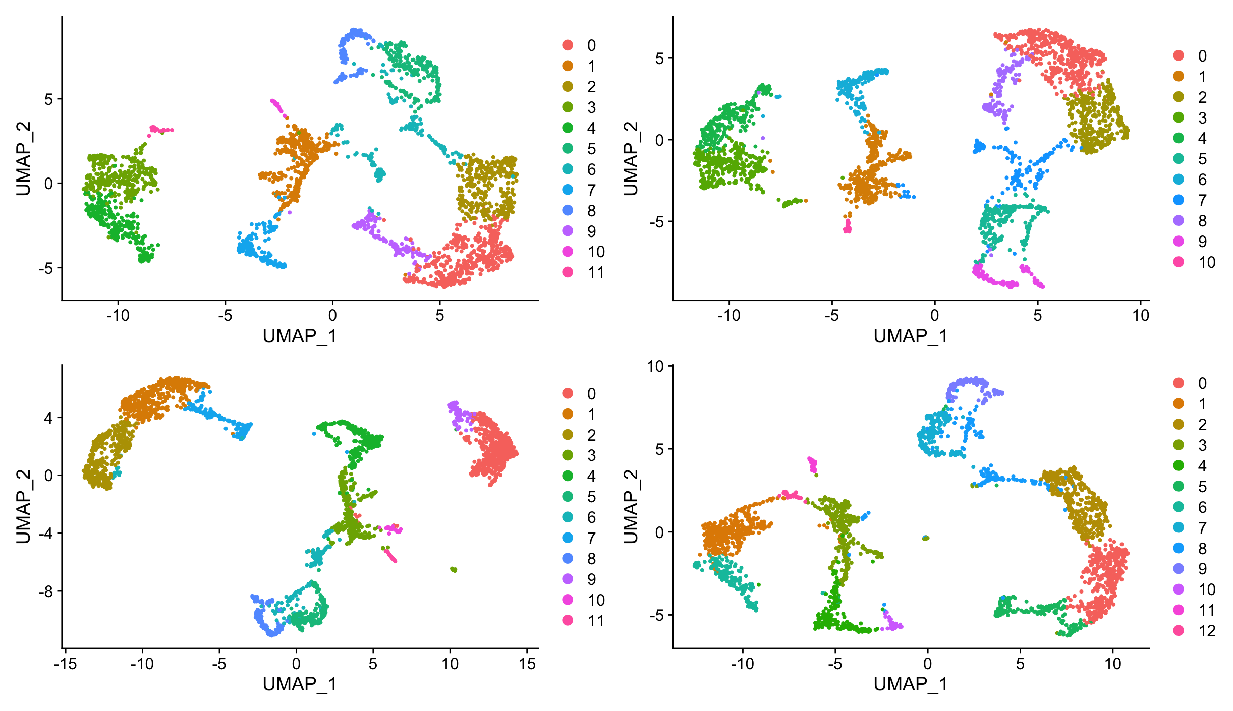
# Visualize UMAPs for comparison
p1 <- DimPlot(visiumSCTmt, reduction = "umap") 
p2 <- DimPlot(visiumSCT, reduction = "umap") 
p3 <- DimPlot(visiumScaleMT, reduction = "umap") 
p4 <- DimPlot(visiumScale, reduction = "umap") 

p1 + p2 + p3 + p4

Result

This will result in four UMAP plots, where the top ones correspond to SCTransform normalization (with and without mitochondrial regression) and the bottom ones correspond to NormalizeData with ScaleData (with and without mitochondrial regression). The left plots include mitochondrial regression, while the right plots do not. You can compare the clustering patterns and overall structure of the data across these different normalization methods to see how they affect the results.

UMAPs from normalised and scaled data. Top left: SCTranscform with regression of mitochondrial genes; top right: SCTranscform without regression; bottom left: Log-normalisation with regression of mitochondrial genes; bottom right: log-normalisation without regression.

We are going to clean up the environment by removing the created Seurat objects with different normalization methods.

rm(visiumSCTmt, visiumSCT, visiumScaleMT, visiumScale)

5.5 Saving the Preprocessed Data

After preprocessing, you can save the Seurat object to disk for future use.

# Save the preprocessed Seurat object
SaveSeuratRds(visium, file = "data/my_preprocessed_mouse_sagittal.rds")

5.6 Loading the Preprocessed Data

We can load the preprocessed object to avoid waiting for the normalization step to complete, as it can take a significant amount of time and memory.

# Load the precomputed preprocessed Seurat object
visium <- LoadSeuratRds(visium, file = "precomputed/preprocessed_mouse_sagittal.rds")

This code provides a basic structure for preprocessing spatial transcriptomics data in Seurat, including scaling, normalization, quality control, and filtering of low-quality cells. You can adapt the parameters based on your specific dataset and analysis requirements.

5.7 Conclusion

Preprocessing spatial transcriptomics data is a critical step in ensuring the quality and reliability of the analysis. By scaling, normalizing, and performing quality control, you can prepare your data for downstream analyses such as clustering, differential expression analysis, and spatial visualization.

5.8 Summary

Key Points

Quality control helps ensure the reliability of the data by filtering out low-quality cells.
Quality control metrics include the number of detected genes, percentage of mitochondrial genes, and total counts per cell.
Scaling and normalization are essential for comparing spatial transcriptomics data across cells and conditions.
Seurat provides functions for scaling, normalization, and quality control of spatial transcriptomics data.