# Load libraries
library(Seurat) # single-cell and spatial analysis toolkit
library(sparseMatrixStats)
library(paletteer) # colour palettes
library(ggplot2) # plotting
library(patchwork) # combining plots

# Load the Seurat object from the previous chapter
visium <- readRDS("precomputed/mouse_brain_normalised_cleaned.rds")7 Dimensionality Reduction
TipLearning Objectives
- Identify highly variable genes for downstream analysis using
SCTransform()orFindVariableFeatures(). - Execute Principal Component Analysis (PCA) using
RunPCA()to reduce data dimensionality. - Interpret elbow plots to determine the appropriate number of principal components to retain.
- Execute UMAP and t-SNE on PCA results to visualise high-dimensional data in two dimensions.
- Explain how the
min.dist,n.neighbors, andperplexityparameters affect the visual structure of non-linear embeddings.
7.1 Setup
We continue working with the sagittal mouse brain dataset from previous chapters.
NoteClick to expand
Start by loading the required libraries and the Seurat object.
As a reminder, this object was created by:
- Importing the raw data using
Load10X_Spatial(), followed by QC and filtering to remove low-quality spots. - Data normalisation using
SCTransform(), which models technical variation and applies variance stabilisation. Stored in the “SCT” assay.
7.2 Dimensionality Reduction
Dimensionality reduction is a standard step when analysing high-dimensional data, such as spatial and single-cell transcriptomics. The main goal is to reduce the gene expression matrix from thousands of genes to a small number of dimensions while retaining most of the variation in the data. These methods identify correlated signals across genes, transforming the data onto a few new axes, thus reducing the dimensionality of the original matrix.
Algorithms generally fall into two categories:
- Linear algorithms: Apply a transformation that preserves the relative distances between the original points (spots or cells).
- Methods include Principal Component Analysis (PCA) and Non-negative Matrix Factorisation (NMF).
- Non-linear algorithms: Exaggerate similarities and differences. Spots that are similar in the original data are placed very close together, while dissimilar spots are pushed further apart.
- Methods include t-Distributed Stochastic Neighbour Embedding (t-SNE) and Uniform Manifold Approximation and Projection (UMAP).
Both strategies are widely used, with two main goals:
- Computational efficiency: Linear transformations like PCA compress the highly dimensional matrices, reducing the computational demand for downstream analyses. Because PCA is linear, it does not distort original distances, but it successfully discards uninformative noise from lowly or randomly expressed genes.
- Visualisation: Non-linear transformations like t-SNE and UMAP are primarily used to plot data in 2D. Because expression patterns are complex, PCA alone cannot capture all nuanced differences in two dimensions. Non-linear methods deal with this complexity better, making them popular for visualisation.
This process typically involves three main steps, illustrated below. We will apply these steps to our mouse brain Visium dataset.

7.3 Feature Selection
Feature selection is the process of identifying highly variable genes (HVGs). Although we could use all genes for PCA, this includes unnecessary noise. Therefore, we remove genes with little variation across spots before performing dimensionality reduction.
There are different approaches for selecting HVGs depending on the assay:
- The
SCTransform()function internally selects highly variable genes based on the residuals from its statistical model. - The
FindVariableFeatures()function selects HVGs from the “Spatial” assay by identifying genes that deviate from the expected mean-variance relationship in the raw counts.
7.3.1 HVGs with sctransform
We can inspect the currently selected variable genes using VariableFeatures():
# Ensure SCT is the active assay
DefaultAssay(visium) <- "SCT"

# See the variable genes
length(VariableFeatures(visium))
[1] 3000head(VariableFeatures(visium))[1] "Ttr" "Mbp" "Hbb-bs" "Plp1" "Ptgds" "Hba-a1"The object currently has 3,000 highly variable genes. These were selected when we ran SCTransform() in the Normalisation chapter.
The ?SCTransform documentation shows an option called variable.features.n. To change the number of variable genes used downstream, we can re-run the normalisation with a new value. For example, to select 2,000 variable genes:
# Re-run SCTransform with 2000 variable genes
visium <- SCTransform(
  visium,
  assay = "Spatial",
  vars.to.regress = "percentMt_Spatial",
  variable.features.n = 2000
)

# Confirm the number of variable genes
length(VariableFeatures(visium))
[1] 2000We can visualise the selected genes using VariableFeaturePlot():
VariableFeaturePlot(visium, assay = "SCT") +
  ggtitle("Highly Variable Genes in SCT Assay")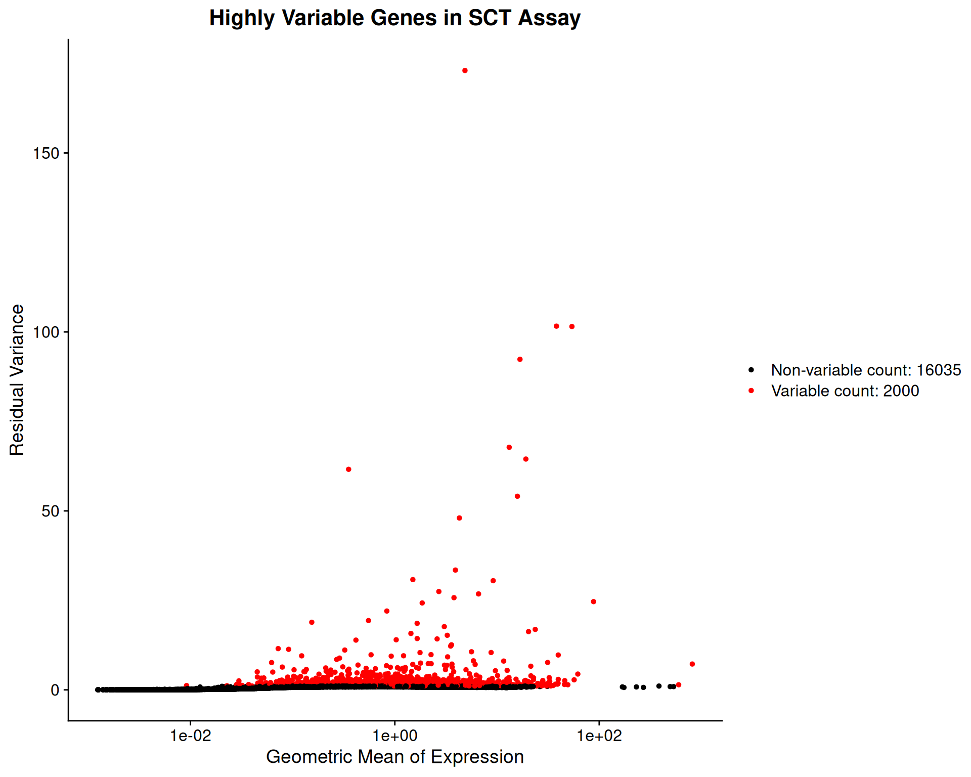
7.3.2 HVGs with FindVariableFeatures()
To identify variable genes in the “Spatial” assay, you can use the FindVariableFeatures() function:
# Ensure Spatial is the active assay
DefaultAssay(visium) <- "Spatial"

# Find variable genes using the "vst" method
visium <- FindVariableFeatures(
  visium,
  assay = "Spatial",
  nfeatures = 2000
)
For clarity, we explicitly set nfeatures = 2000 here, but this is the default value if you don’t specify it.
We can use the same function as before visualise the variable genes for the “Spatial” assay:
VariableFeaturePlot(visium, assay = "Spatial") +
  ggtitle("Highly Variable Genes in Spatial Assay")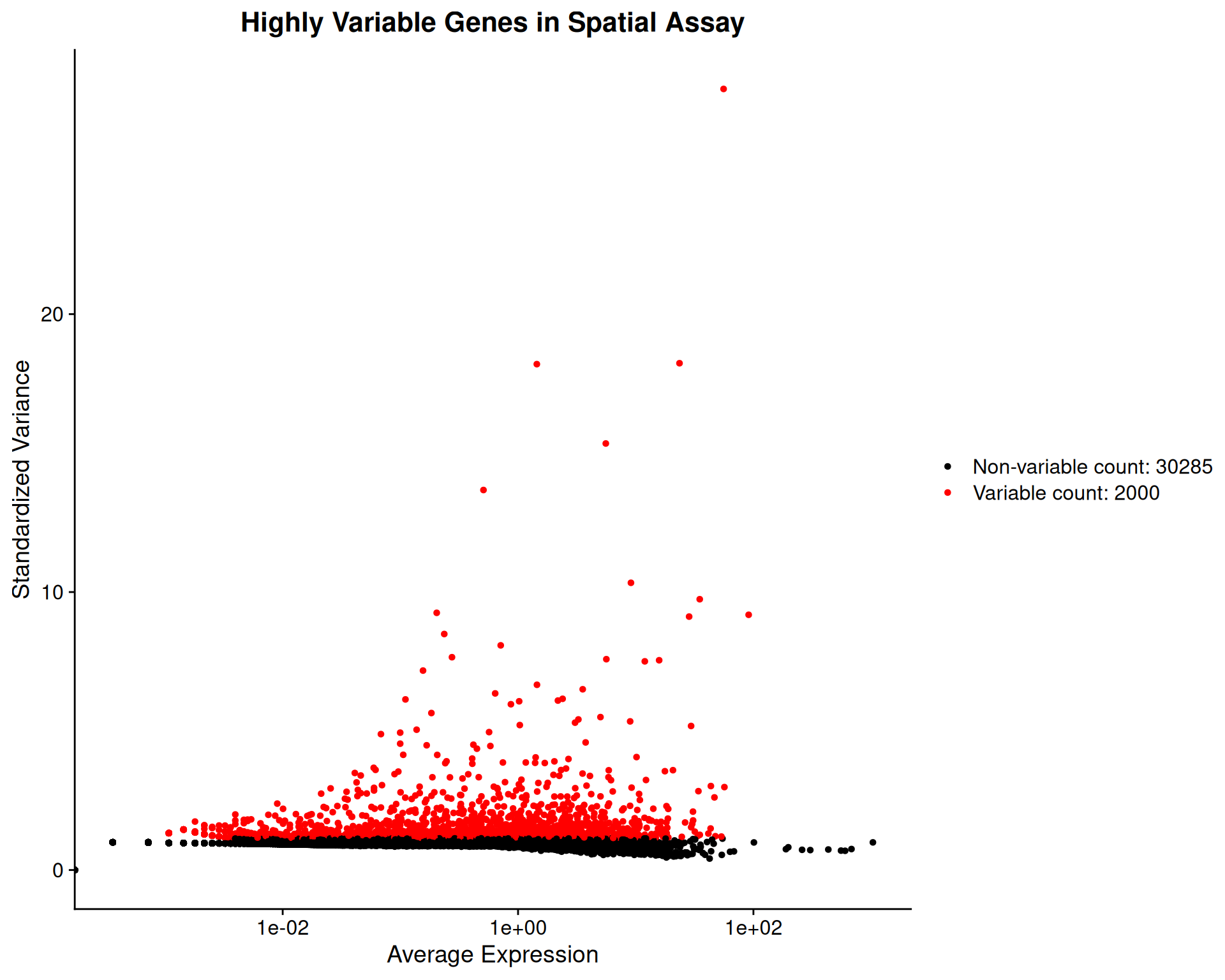
7.4 Principal Component Analysis (PCA)
Having selected highly variable genes, we can perform dimensionality reduction. We use the “SCT” assay for the rest of our analysis.
# Set the default assay to SCT
DefaultAssay(visium) <- "SCT"
Principal Component Analysis (PCA) reduces the dimensionality of the data while retaining most of the variance. We use RunPCA() to compute the principal components:
# Perform PCA on the SCT assay
visium <- RunPCA(visium, assay = "SCT", npcs = 100)

# Confirm a dimensionality reduction called "pca" has been added to the object
visium
We specify npcs = 100 to compute the first 100 principal components. The default is 50, but calculating more allows us to observe how the variance explained changes across a wider range of dimensions.
To decide how many principal components (PCs) to retain for downstream analyses, we examine an elbow plot. This plot shows the percentage of variance explained by each PC.
# Check elbow plot to determine the number of PCs
ElbowPlot(visium, ndims = 100, plot_type = "variance", reduction = 'pca')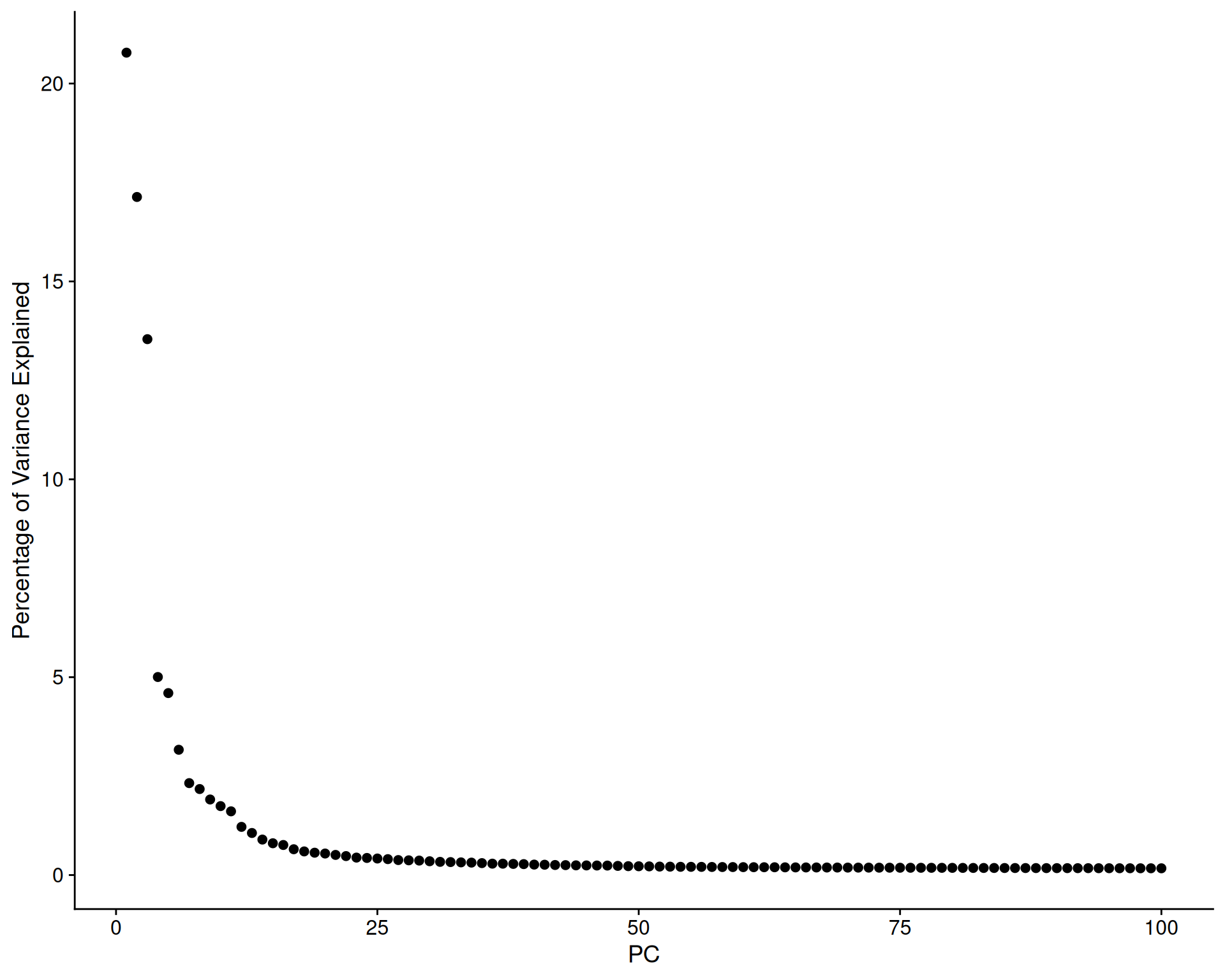
The variance explained drops sharply after the first few PCs, then levels off, creating a characteristic “elbow” shape.
A cumulative variance plot shows the total variance explained by the first n PCs:
# Get the variance explained by each PC
ElbowPlot(
  visium,
  ndims = 100,
  plot_type = "cumulative_variance",
  reduction = 'pca'
) +
  geom_hline(yintercept = 90) +
  geom_vline(xintercept = 50)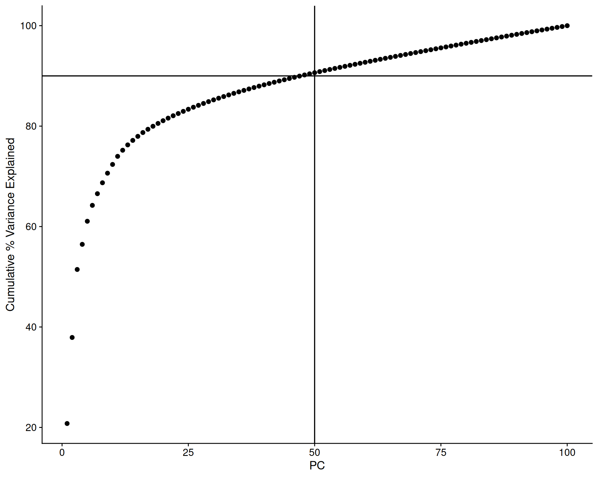
We’ve added some marker lines to help us decide how many PCs to use. We can see that the first 50 PCs explain just over 90% of the total variance. This suggests that such a threshold captures most of the signal while heavily reducing the dataset dimensionality. We go from 18035 genes down to 50 dimensions.
As we are happy with 50 PCs, we re-run the PCA with npcs = 50:
# Perform PCA on the SCT assay with 50 PCs
visium <- RunPCA(visium, assay = "SCT", npcs = 50)
7.5 UMAP and t-SNE
Uniform Manifold Approximation and Projection (UMAP) and t-Distributed Stochastic Neighbour Embedding (t-SNE) are non-linear dimensionality reduction techniques well-suited for visualising high-dimensional data in 2D.
They are run on the PCA results to further compress dimensionality for visualisation. The RunUMAP() and RunTSNE() functions compute the embeddings and add them to the Seurat object.
# Perform UMAP on the PCA results
visium <- RunUMAP(visium, reduction = "pca", dims = 1:50)

# Perform t-SNE on the PCA results
visium <- RunTSNE(visium, reduction = "pca", dims = 1:50)

# Confirm these were added to the object
Reductions(visium)
[1] "pca" "umap" "tsne"You can use the DimPlot() function to visualise these reductions. We plot both side-by-side for comparison:
# UMAP plot
umap <- DimPlot(visium, reduction = "umap") +
  ggtitle("UMAP") +
  theme(legend.position = "none")

# t-SNE plot
tsne <- DimPlot(visium, reduction = "tsne") +
  ggtitle("t-SNE") +
  theme(legend.position = "none")

# Visualise both
umap + tsne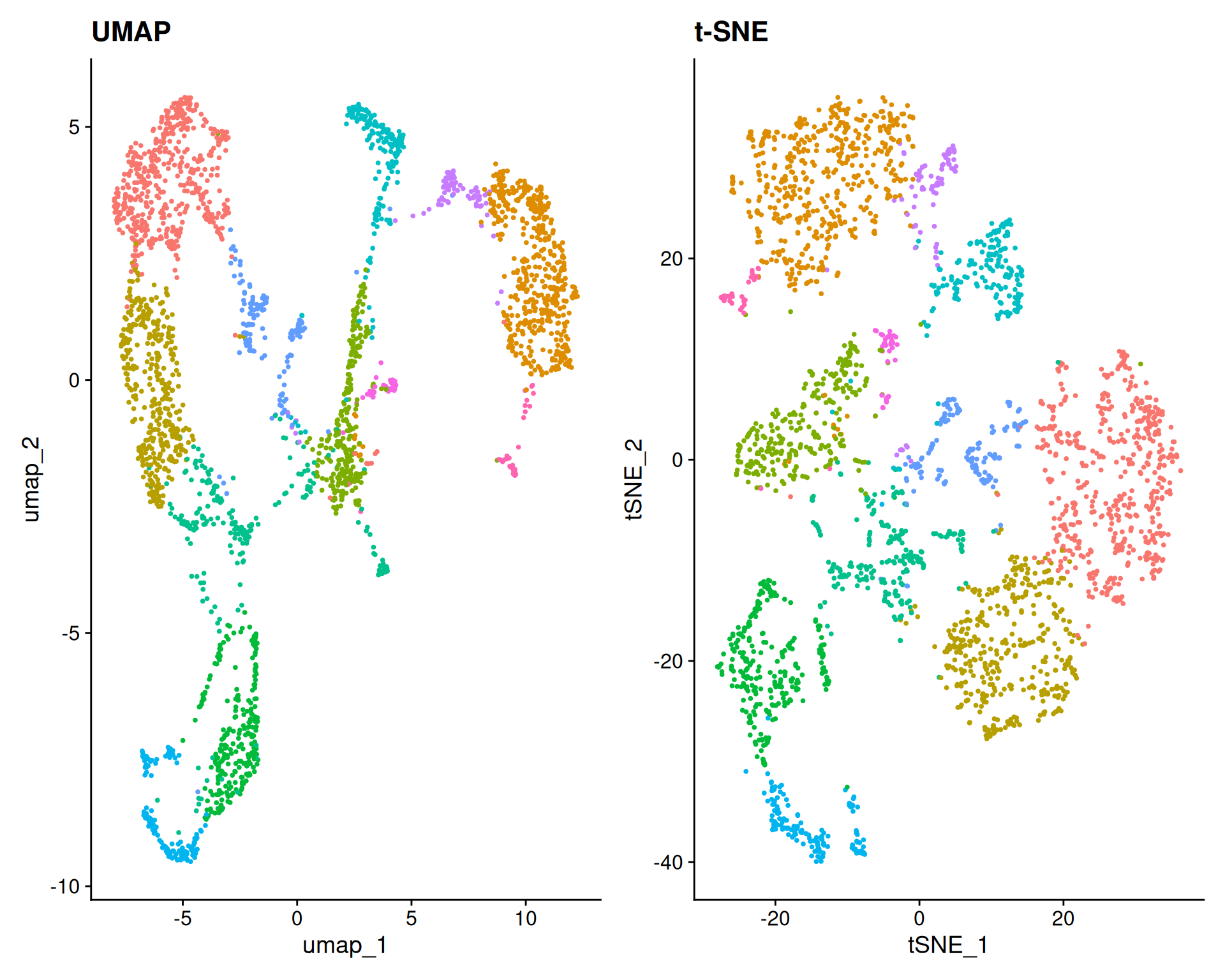
These plots show the UMAP and t-SNE embeddings, with each point representing a spatial spot. Although we have not yet identified clusters or cell types, you can already see some structure likely corresponding to distinct anatomical regions in the brain.
TipUMAP or t-SNE?
UMAP is generally preferred over t-SNE, but comparing them can still be informative.
UMAP preserves global relationships better, showing how clusters relate continuously.
t-SNE emphasises local relationships, often creating distinct, separated clusters. This can falsely suggest that clusters are highly isolated. However, by preserving local neighbourhood structures, t-SNE can help identify small subpopulations within the data.
7.6 UMAP Parameters
UMAP offers parameters to control the balance between local and global structure. Two important parameters are:
n.neighbors: The size of the local neighbourhood used for the projection.min.dist: The minimum distance allowed between points in the low-dimensional space.
To explore these parameters, we first vary min.dist while keeping n.neighbors at the default value of 30. We use reduction.name and reduction.key to store each result separately, to avoid overwriting the default “umap” slot.
# Default n.neighbors but high min.dist
visium <- RunUMAP(
  visium,
  reduction = "pca",
  dims = 1:50,
  n.neighbors = 30,
  min.dist = 0.5,
  reduction.name = "umap_highdist",
  reduction.key = "UMAPH"
)

# Default n.neighbors but low min.dist
visium <- RunUMAP(
  visium,
  reduction = "pca",
  dims = 1:50,
  n.neighbors = 30,
  min.dist = 0.01,
  reduction.name = "umap_lowdist",
  reduction.key = "UMAPL"
)

# Visualise side-by-side
umapHighDist <- DimPlot(visium, reduction = "umap_highdist") +
  ggtitle("min.dist = 0.5") +
  theme(legend.position = "none")
umapLowDist <- DimPlot(visium, reduction = "umap_lowdist") +
  ggtitle("min.dist = 0.01") +
  theme(legend.position = "none")

umapHighDist + umapLowDist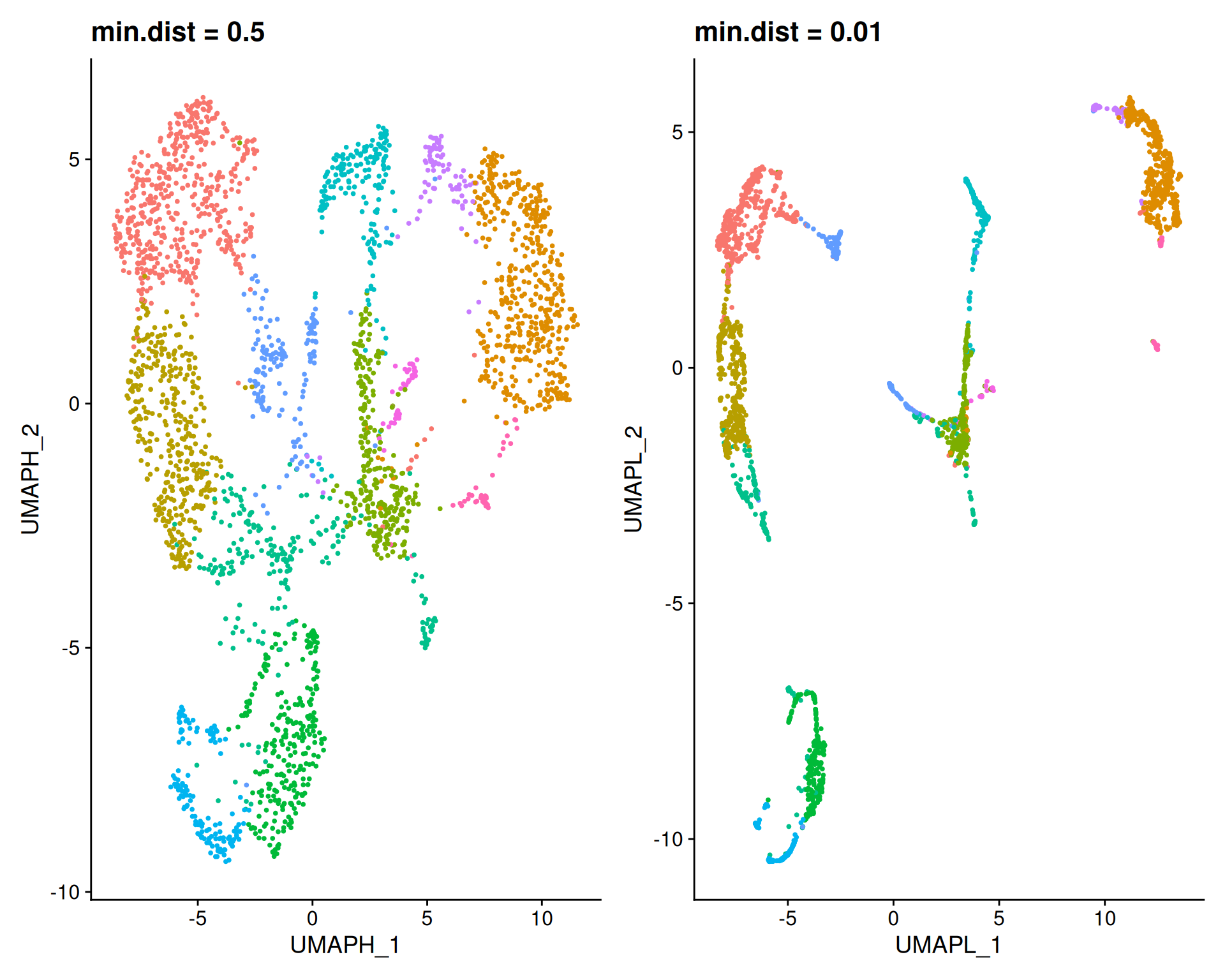
A high min.dist (0.5) forces points apart, resulting in a diffuse plot that highlights global structure. A low min.dist (0.01) allows points to pack tightly. You may notice that the overall layout is actually very similar between these two plots. The main difference is how strongly the points repel each other.
Next, we vary n.neighbors, keeping min.dist at the default value of 0.3:
# Default min.dist but high n.neighbors
visium <- RunUMAP(
  visium,
  reduction = "pca",
  dims = 1:50,
  n.neighbors = 100,
  min.dist = 0.3,
  reduction.name = "umap_highnn",
  reduction.key = "UMAPHN"
)

# Default min.dist but low n.neighbors
visium <- RunUMAP(
  visium,
  reduction = "pca",
  dims = 1:50,
  n.neighbors = 5,
  min.dist = 0.3,
  reduction.name = "umap_lownn",
  reduction.key = "UMAPLN"
)

# Visualise side-by-side
umapHighNeighbours <- DimPlot(visium, reduction = "umap_highnn") +
  ggtitle("n.neighbors = 100") +
  theme(legend.position = "none")
umapLowNeighbours <- DimPlot(visium, reduction = "umap_lownn") +
  ggtitle("n.neighbors = 5") +
  theme(legend.position = "none")

umapHighNeighbours + umapLowNeighbours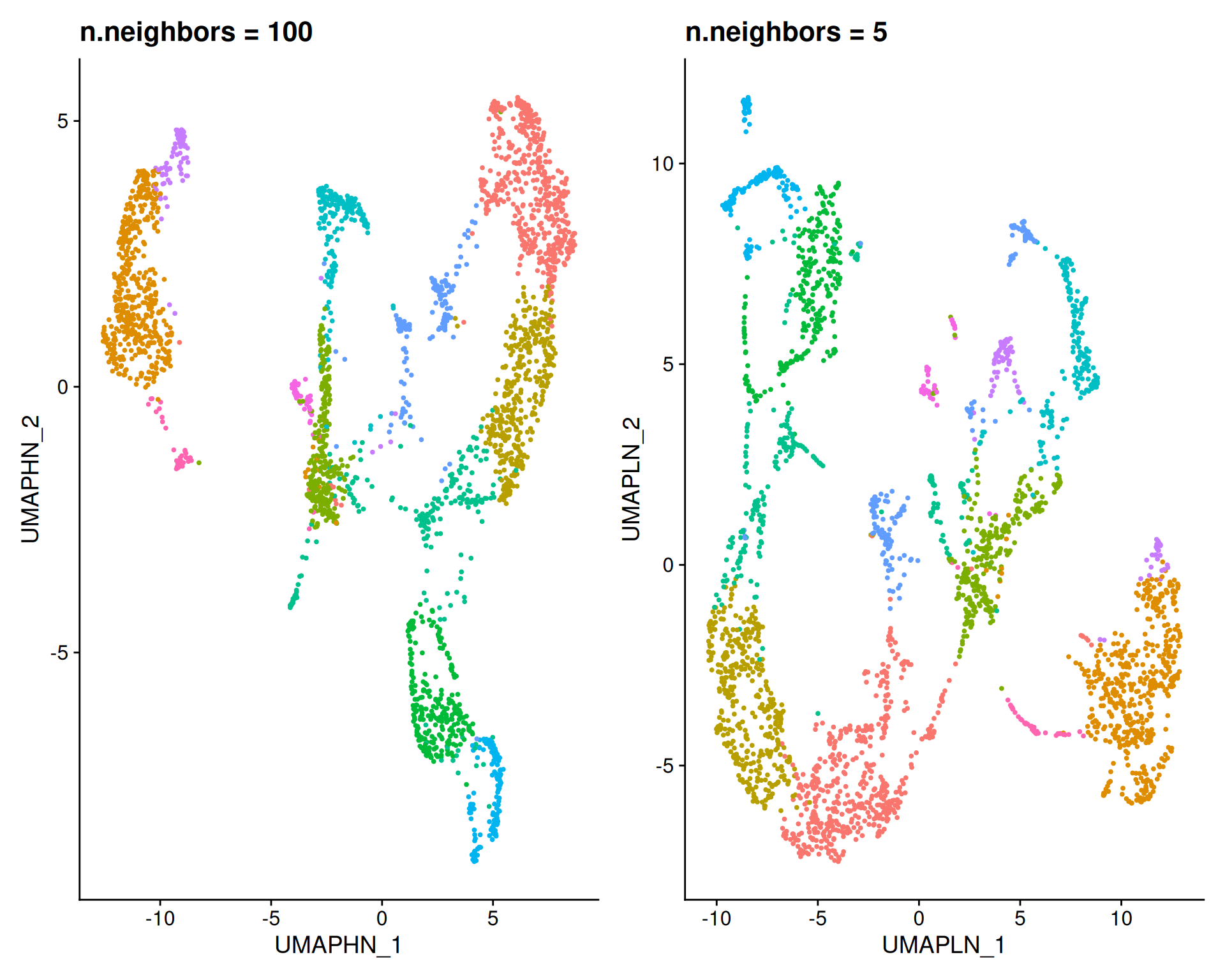
A high n.neighbors (100) captures global structure, forming large, clearly separated groups that reveal broad patterns. A low n.neighbors (5) captures fine local structure, breaking the data into many small clusters. This can help to identify small subpopulations.
7.7 t-SNE Parameters
For t-SNE, the perplexity parameter controls the balance between local and global structure, similarly to n.neighbors in UMAP.
The default is perplexity = 30. We can test different values to see their impact:
# Perform tSNE with different values for perplexity
visium <- RunTSNE(
  visium,
  reduction = "pca",
  dims = 1:30,
  perplexity = 100,
  reduction.name = "tsne_highperp",
  reduction.key = "TSNEHP"
)
visium <- RunTSNE(
  visium,
  reduction = "pca",
  dims = 1:30,
  perplexity = 5,
  reduction.name = "tsne_lowperp",
  reduction.key = "TSNELP"
)

# Visualise the tSNE results with different parameters
tsneHighPerp <- DimPlot(visium, reduction = "tsne_highperp") +
  ggtitle("perplexity = 100") +
  theme(legend.position = "none")
tsneLowPerp <- DimPlot(visium, reduction = "tsne_lowperp") +
  ggtitle("perplexity = 5") +
  theme(legend.position = "none")

tsneHighPerp + tsneLowPerp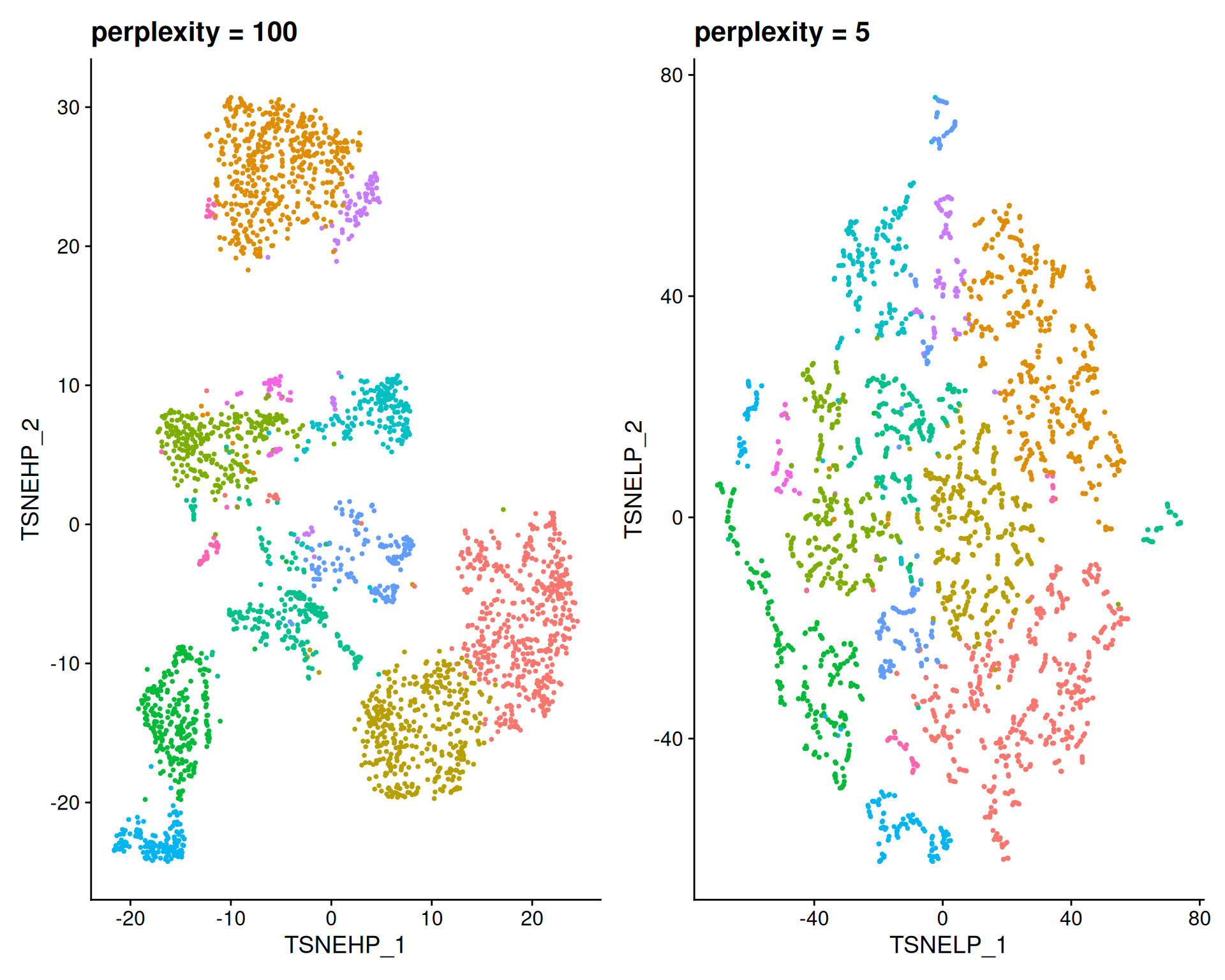
- A high
perplexity(100) creates larger groups, capturing global structure and broad patterns. - A low
perplexity(5) creates small, fragmented clusters, capturing fine local structure.
7.8 Exporting the Object
We save the Seurat object for use in the next chapter.
To make the objects smaller and save memory in downstream steps, we remove the extra dimensionality reduction tables. However, you may want to keep these if you plan to use them for other analyses or visualisations later on.
# Check which dimensionality reductions we have in the object
Reductions(visium)
[1] "pca" "umap" "tsne" "umap_highdist"
[5] "umap_lowdist" "umap_highnn" "umap_lownn" "tsne_highperp"
[9] "tsne_lowperp" # Remove those we don't want to keep
visium[["umap_highdist"]] <- NULL
visium[["umap_lowdist"]] <- NULL
visium[["umap_highnn"]] <- NULL
visium[["umap_lownn"]] <- NULL
visium[["tsne_highperp"]] <- NULL
visium[["tsne_lowperp"]] <- NULL
# Confirm they have been removed
Reductions(visium)[1] "pca" "umap" "tsne"Finally, save the object:
# Save the cleaned object for future use
saveRDS(visium, "results/mouse_brain_dimred.rds")
7.9 Summary
TipKey Points
- Seurat provides functions to identify highly variable genes (HVGs) before dimensionality reduction.
SCTransform()selects features using thevariable.features.nargument.FindVariableFeatures()identifies features for the “Spatial” assay using thenfeaturesargument.
- Principal Component Analysis (PCA) is a linear method that compresses the highly dimensional gene expression matrix into fewer dimensions.
- The
RunPCA()function calculates principal components on Seurat object.
- The
- The variance explained by each principal component help determine how many PCs capture the majority of the data’s variance.
- The
ElbowPlot()function can be used to visualise the variance explained by each principal component.
- The
- Non-linear dimensional reductions like UMAP and t-SNE are used primarily to visualise complex patterns in two dimensions.
RunUMAP()andRunTSNE()compute these embeddings, whileDimPlot()visualises the results.
- Parameters in UMAP and t-SNE control the balance between local and global structure.
min.distin UMAP determines how tightly points are allowed to pack together.n.neighborsin UMAP andperplexityin t-SNE determine the size of the local neighbourhood, where higher values reveal broader global patterns and lower values highlight small local clusters.