# Load libraries
library(Seurat) # single-cell and spatial analysis toolkit
library(sparseMatrixStats)
library(paletteer) # colour palettes
library(ggplot2) # plotting
library(patchwork) # combining plots

# Load the Seurat object from the previous chapter
visium <- readRDS("precomputed/mouse_brain_filtered.rds")6 Normalisation
TipLearning Objectives
- Explain why normalisation is needed in spatial transcriptomics data, including the roles of library size variation and confounders such as mitochondrial fraction.
- Apply
SCTransform()andNormalizeData()+ScaleData()to a Visium dataset. - Describe the data layers stored in a Seurat assay after normalisation and switch between assays.
- Compare normalisation methods by running clustering on each normalised dataset and calculating the Adjusted Rand Index (ARI) between cluster assignments.
- Interpret published benchmarking evidence to help choosing suitable normalisation methods for spatial data.
6.1 Setup
NoteClick to expand
We continue with the Visium mouse brain dataset from 10x Genomics.
Start by loading the required libraries and reading the Seurat object from the previous chapter.
This object was created by:
- Importing the raw data using
Load10X_Spatial() - Removing spots where:
- The library size was less than 1000 (
nCount_Spatial < 1000) - The number of detected genes was less than 500 (
nFeature_Spatial < 500) - The percentage of mitochondrial counts was greater than 30 (
percentMt_Spatial > 30)
- The library size was less than 1000 (
6.2 Normalistaion Overview
Normalisation makes expression values comparable across spots and, when relevant, across samples.
One important source of technical variation is library size, i.e. the total number of reads per spot. When library sizes differ, raw counts can make spots look biologically different even when they are transcriptomically similar. For example, if two identical spots are sequenced at different depths, the deeper spot will appear to have higher expression for most genes.
Other confounders can also affect observed expression. For instance, a high mitochondrial fraction can shift reads away from other genes, making those genes appear under-expressed.
If we do not adjust for these effects, clustering can reflect technical artefacts rather than biology.
Normalisation remains an active research area, and no single method works best for every dataset. The key challenge is balancing technical correction with biological signal retention.
Many workflows apply single-cell normalisation methods to spatial data by treating each spot as a cell-like unit. Some common methods include:
- sctransform: Fits a negative binomial regression model to normalise raw counts, accounting for library size differences across spots and any specified confounders. This is the default recommendation in Seurat tutorials.
- Library size normalisation: This is a relatively simple normalisation where each count is divided by the total counts for the respective spot (i.e. the spot’s library size), followed by a log transformation. A pseudocount of 1 is added to the counts to avoid \(log(0) = Inf\).
- Scran normalisation: Instead of using the spot library size as the scaling factor, this method determines size factors for each spot by pooling information across similar spots, using methods inspired by bulk RNA-seq normalisation. This method can help to improve normalisation in sparse datasets such as single-cell and spatial transcriptomics data. The method is implemented in the
scranandscuttlepackages.
These methods all assume that spots behave like single cells. Newer methods, such as SpaNorm, aim to make normalisation spatially aware.
In this chapter, we compare sctransform and library size normalisation, as they are both readily available in Seurat. We also briefly mention scran and SpaNorm normalisation methods.
6.3 sctransform
The sctransform normalisation is available through the SCTransform() function in Seurat. This method fits a negative binomial model to account for library size differences and optional confounders such as mitochondrial percentage.
Seurat vignettes recommend this method, although recent benchmarking suggests it may not always be ideal for spatial data (discussed below).
SCTransform() also applies variance stabilisation. Before normalisation, you can see the usual mean-variance trend in count data: genes with higher mean expression also show higher variance.
# extract the raw counts
rawCts <- as.matrix(visium[["Spatial"]]$counts)

# plot the mean-variance relationship
plot(rowMeans(rawCts), rowVars(rawCts), log = "xy")
abline(0, 1, col = "red")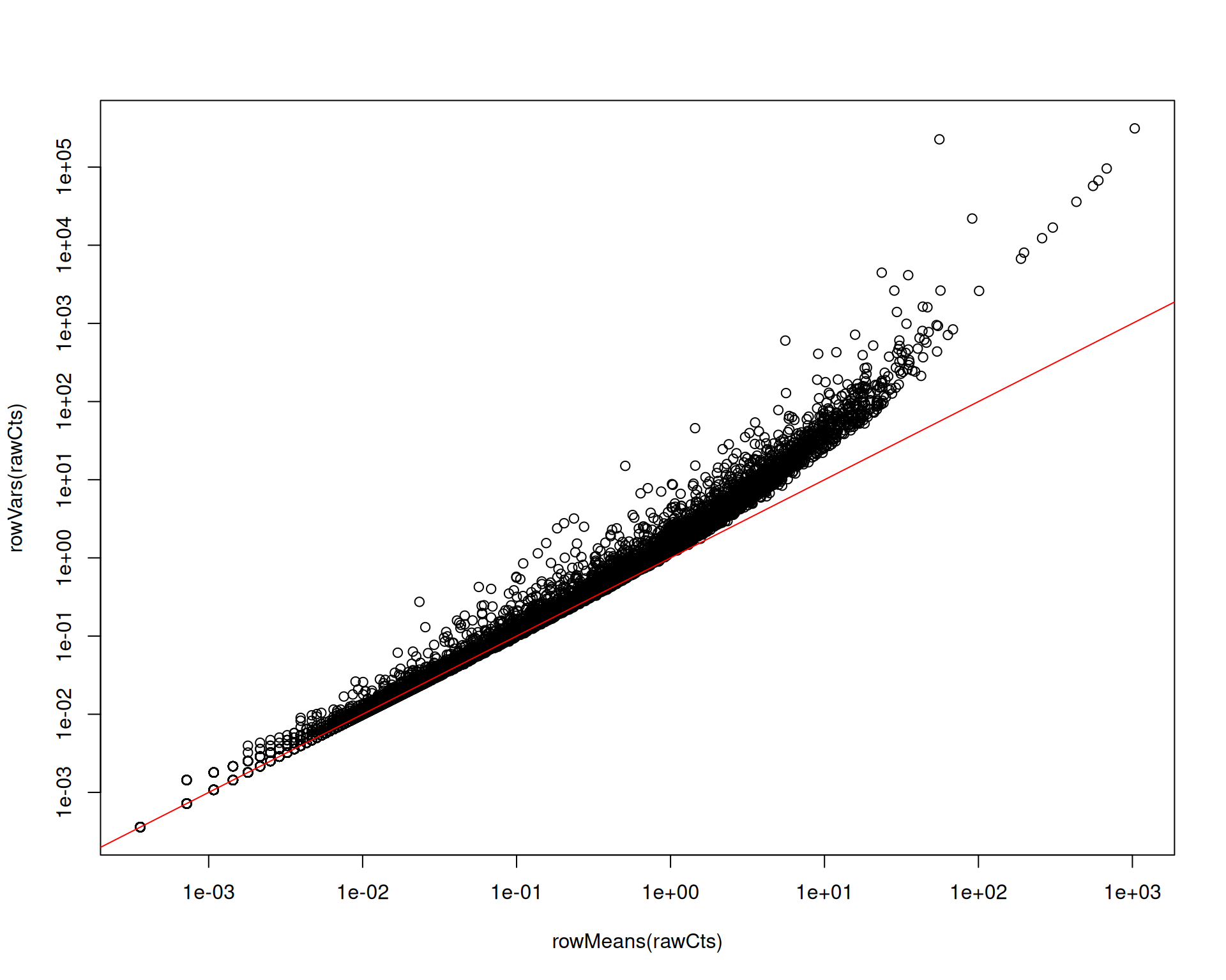
Removing this trend reduces the risk that highly expressed genes dominate variable-feature selection and bias downstream steps such as PCA.
A key argument is vars.to.regress, which removes variation linked to metadata variables such as mitochondrial percentage.
# Perform SCTransform normalisation
visium <- SCTransform(
  visium,
  assay = "Spatial",
  vars.to.regress = "percentMt_Spatial"
)

# View the object
visium
An object of class Seurat
50320 features across 2780 samples within 2 assays
Active assay: SCT (18035 features, 3000 variable features)
3 layers present: counts, data, scale.data
1 other assay present: Spatial
1 spatial field of view present: slice1After SCTransform(), Seurat sets SCT as the default assay. This matters because downstream functions will now use SCT unless you switch assays explicitly.
The SCT assay contains three layers:
counts: model-corrected counts (adjusted for library size and any regressed variables). These are reconstructed from the fitted model.data: log-transformed counts with an added pseudocount of 1 (to avoid \(log(0) = Inf\)).scale.data: model residuals, which represent corrected expression on a continuous scale. Downstream steps such as dimensionality reduction and clustering use this layer.
If you plot mean versus variance in scale.data, the strong trend is largely removed, as expected after variance stabilisation:
# Extract the variance-stabilised data from SCTransform
sctScaleData <- as.matrix(visium[["SCT"]]$scale.data)
plot(rowMeans(sctScaleData), rowVars(sctScaleData))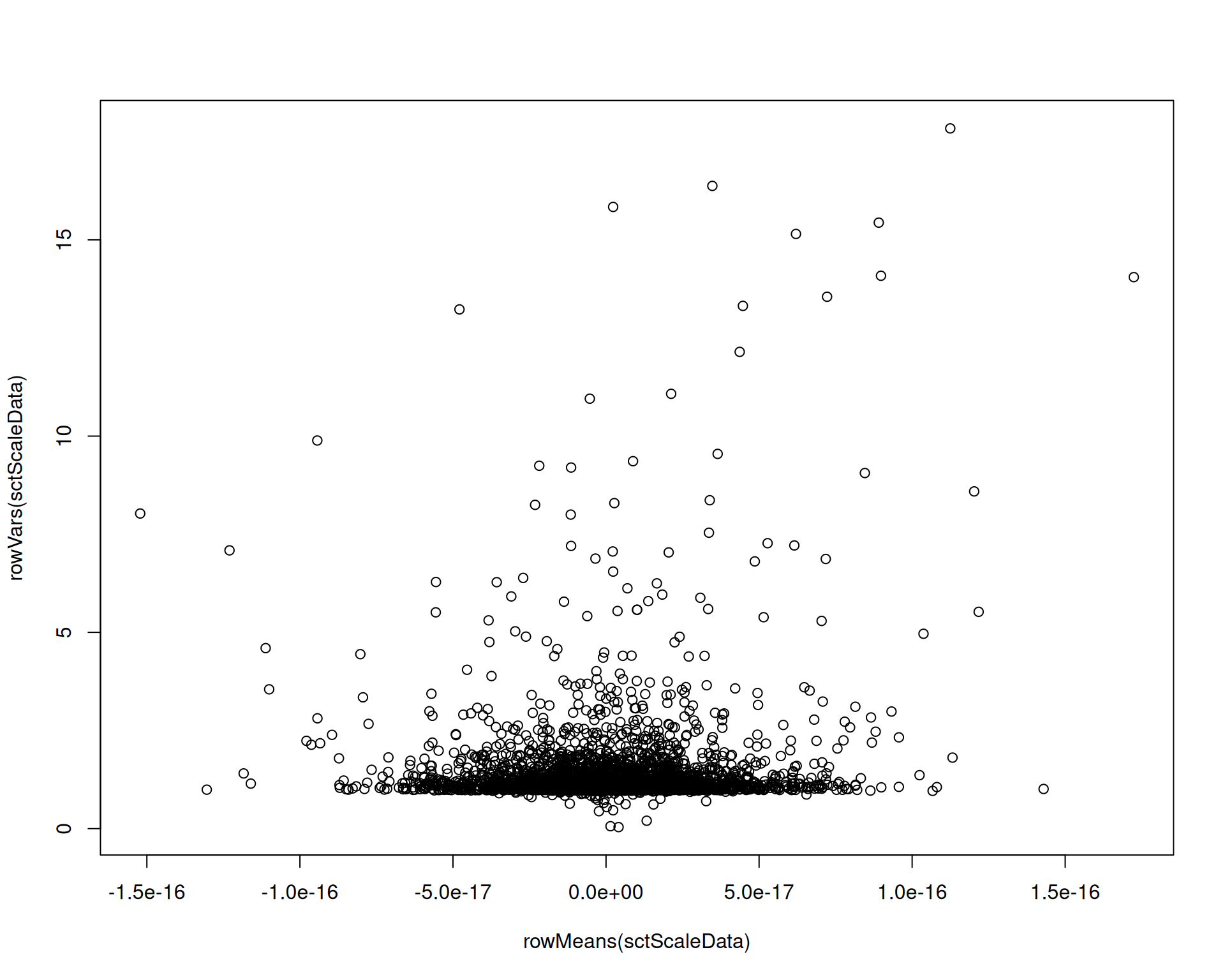
As a result, highly expressed genes are less likely to dominate downstream feature selection.
TipManaging memory usage by
SCTransform
SCTransform() can use substantial RAM on larger datasets. To reduce memory pressure:
- By default, the function uses 5000 cells (spots here) to estimate model parameters. You can reduce this with
ncells(for example, 2000) to lower memory usage, at the cost of less stable parameter estimates. - Setting
conserve.memory = TRUEreduces memory usage, but usually increases runtime because data are reloaded repeatedly during fitting. - If you have access to a compute cluster, run this step on a high-memory node. Save the object after normalisation so later steps can start from the pre-normalised file.
6.4 Library size normalisation
A simpler alternative is Seurat’s NormalizeData(), which applies three steps:
- Divides the counts for each gene by the total counts for that spot (its library size).
- Multiplies by a scale factor (default 10,000) to avoid very small values.
- Log-transforms the scaled values.
You should apply NormalizeData() to the raw counts in the Spatial assay, not to SCT. You can do this in two ways:
- Change the default assay with
DefaultAssay(visium) <- "Spatial"before running the function. - Specify the assay in the function call with
assay = "Spatial".
# Perform log-normalisation only
visium <- NormalizeData(visium, assay = "Spatial")

# Confirm a new layer called "data" has been added to the "Spatial" assay
visium[["Spatial"]]
Assay (v5) data with 32285 features for 2780 cells
First 10 features:
Xkr4, Gm1992, Gm19938, Gm37381, Rp1, Sox17, Gm37587, Gm37323, Mrpl15,
Lypla1
Layers:
counts, data NormalizeData() adds a data layer to Spatial containing log-normalised values.
Although simple, this approach often performs well for tasks such as dimensionality reduction and clustering, so it remains widely used.
Log-normalisation does weaken the mean-variance trend, though usually less effectively than SCTransform():
# Extract the log-normalised data
logCts <- as.matrix(visium[["Spatial"]]$data)
plot(rowMeans(logCts), rowVars(logCts))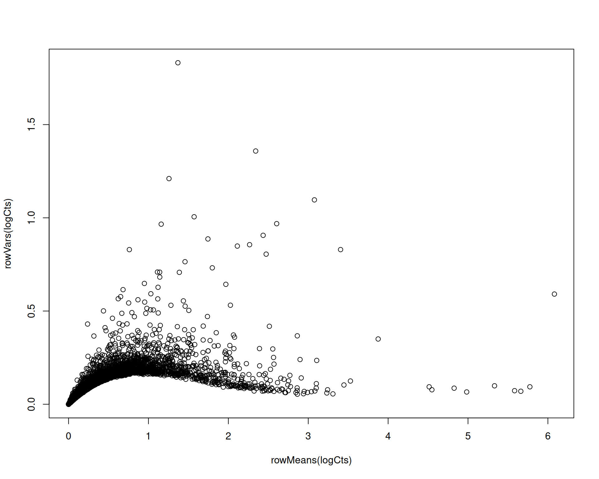
6.4.1 Scaling and confounder regression
Seurat often follows log-normalisation with ScaleData(). This function has two main roles:
- Scaling: a Z-score transformation where each gene is mean-centred and divided by its standard deviation.
- Regressing out confounders: removes variation associated with metadata variables such as mitochondrial percentage.
Scaling reduces the influence of absolute expression magnitude in downstream analyses because values are expressed as per-gene Z-scores.
There is a trade-off: scaling can also amplify noise in lowly expressed genes. You can disable Z-scoring with do.scale = FALSE, do.center = FALSE, although this is not Seurat’s default.
ScaleData() can also regress confounders, but this workflow is much slower than SCTransform() on large objects. To keep this chapter practical, we provide a preprocessed object and include the full code in a collapsed section.
ScaleData() is used after NormalizeData(). We already ran log-normalisation above; here we show both steps together for completeness.
Show code for normalisation and scaling - takes a long time to run!
# Perform log-normalisation and scaling
# This takes a long time to run!
# Read the preprocessed object below instead
visium <- visium |>
  NormalizeData(assay = "Spatial") |>
  ScaleData(assay = "Spatial", vars.to.regress = "percentMt_Spatial")
# Read the preprocessed object with log-normalisation and scaling already applied
visium <- readRDS("precomputed/mouse_brain_normalised.rds")
# Confirm a new layer called "scale.data" has been added to the "Spatial" assay
visium[["Spatial"]]This adds a scale.data layer to Spatial, containing log-normalised and scaled values.
TipThe
scale.data layer
Some Seurat functions expect a scale.data layer in the active assay.
If you want to keep log-normalised values without Z-scoring or regression, run ScaleData() with do.scale = FALSE, do.center = FALSE and no regression terms. This effectively copies data into scale.data, which satisfies functions that require that layer.
6.5 Scran normalisation
In simple library-size normalisation, each spot is scaled by its total counts. Scran instead estimates spot-specific size factors by pooling information across similar spots, which can improve robustness in sparse data such as single-cell and spatial transcriptomics.
The scran workflow is built for Bioconductor classes such as SingleCellExperiment and SpatialExperiment. In Seurat, we therefore need to run the key steps manually.
As this is a fairly involved process, we provide the step-by-step instructions in the Extended Materials for those interested: Scran normalisation.
6.6 SpaNorm
The methods above are not spatially aware because they ignore spot coordinates. Recent work suggests this can be problematic, as library size can vary with spatial location. If so, correcting library size without spatial context may over-correct and remove true biological structure.
This is still an active research area, so available tools are limited. SpaNorm is one of the few available options.
At the time of writing, a known bug prevents direct use with our Seurat object. We include the code below to show the intended workflow and link to the current status (GitHub issue).
# NOTE: this code is for reference only, it currently does not work

# create a separate assay for the SpaNorm normalisation
visium[["SpaNorm"]] <- CreateAssayObject(counts = visium[["Spatial"]]$counts)
DefaultAssay(visium) <- "SpaNorm"

# Perform SpaNorm normalisation - currently fails due to bug
visium <- SpaNorm::SpaNorm(visium)

# check the new assay
visium[["SpaNorm"]]
6.7 Which Normalisation?
There is no universal answer for which normalisation to choose.
Bhuva et al. (2024) benchmarked several non-spatial normalisation and clustering workflows across tissues and technologies. One key conclusion was:
(…) library size or total detections per cell significantly differ across tissue structures, representing real biology rather than technical variation.
This implies that methods that aggressively correct library size can remove genuine biological signal. In that benchmark, SCTransform performed worse than scran and simple library-size normalisation (equivalent to NormalizeData() without Z-scoring).
In follow-up work, Salim et al. (2025) reported that SpaNorm better removed technical variation while preserving biological structure. They also found that SCTransform tended to preserve spatial domains less effectively than scran and standard library-size normalisation.
These benchmarks are still limited in scope, so a practical strategy is to compare several methods and check whether your biological conclusions are robust.
6.8 Comparing normalisation strategies
So far, we applied:
SCTransform()normalisation with variance stabilising transform- Library size log-normalisation and Z-score scaling (
NormalizeData()+ScaleData())
In both cases, we regressed out mitochondrial percentage as a confounder.
To compare methods, we run the same quick clustering workflow for each normalisation and visualise the cluster labels on the tissue image. We will cover clustering in depth in a later chapter. Here the goal is method comparison, so don’t worry too much about the details of the implementation.
# SCTransform with mitochondrial regression
DefaultAssay(visium) <- "SCT"
visium <- visium |>
  RunPCA() |>
  FindNeighbors(dims = 1:30) |>
  FindClusters(resolution = 0.5, cluster.name = "sctClusters")

# Library size normalisation with scaling and mitochondrial regression
DefaultAssay(visium) <- "Spatial"
visium <- visium |>
  FindVariableFeatures() |>
  RunPCA() |>
  FindNeighbors(dims = 1:30) |>
  FindClusters(resolution = 0.5, cluster.name = "scaledClusters")
The main result of interest to us are two new columns added to the metadata, sctClusters and scaledClusters, which contain the cluster labels for each normalisation method.
# View the metadata to confirm the new cluster columns
head(visium[[]])
orig.ident nCount_Spatial nFeature_Spatial
AAACAAGTATCTCCCA-1 SeuratProject 18286 4736
AAACACCAATAACTGC-1 SeuratProject 9311 3735
AAACAGAGCGACTCCT-1 SeuratProject 36450 7285
AAACAGCTTTCAGAAG-1 SeuratProject 30800 7298
AAACAGGGTCTATATT-1 SeuratProject 27617 6892
AAACATTTCCCGGATT-1 SeuratProject 38072 7476
percentMt_Spatial nCountFiltered percentMtFiltered
AAACAAGTATCTCCCA-1 15.432571 FALSE FALSE
AAACACCAATAACTGC-1 14.391580 FALSE FALSE
AAACAGAGCGACTCCT-1 13.242798 FALSE FALSE
AAACAGCTTTCAGAAG-1 9.681818 FALSE FALSE
AAACAGGGTCTATATT-1 11.721041 FALSE FALSE
AAACATTTCCCGGATT-1 10.532675 FALSE FALSE
nFeatureFiltered combinedFiltered nCount_SCT nFeature_SCT
AAACAAGTATCTCCCA-1 FALSE FALSE 19553 4695
AAACACCAATAACTGC-1 FALSE FALSE 18547 4223
AAACAGAGCGACTCCT-1 FALSE FALSE 21438 6474
AAACAGCTTTCAGAAG-1 FALSE FALSE 21608 7049
AAACAGGGTCTATATT-1 FALSE FALSE 21638 6766
AAACATTTCCCGGATT-1 FALSE FALSE 21652 6501
scranSizeFactors sctClusters scaledClusters
AAACAAGTATCTCCCA-1 0.8139093 2 3
AAACACCAATAACTGC-1 0.4757088 4 4
AAACAGAGCGACTCCT-1 1.8205740 1 2
AAACAGCTTTCAGAAG-1 1.8627597 9 7
AAACAGGGTCTATATT-1 1.6270190 9 7
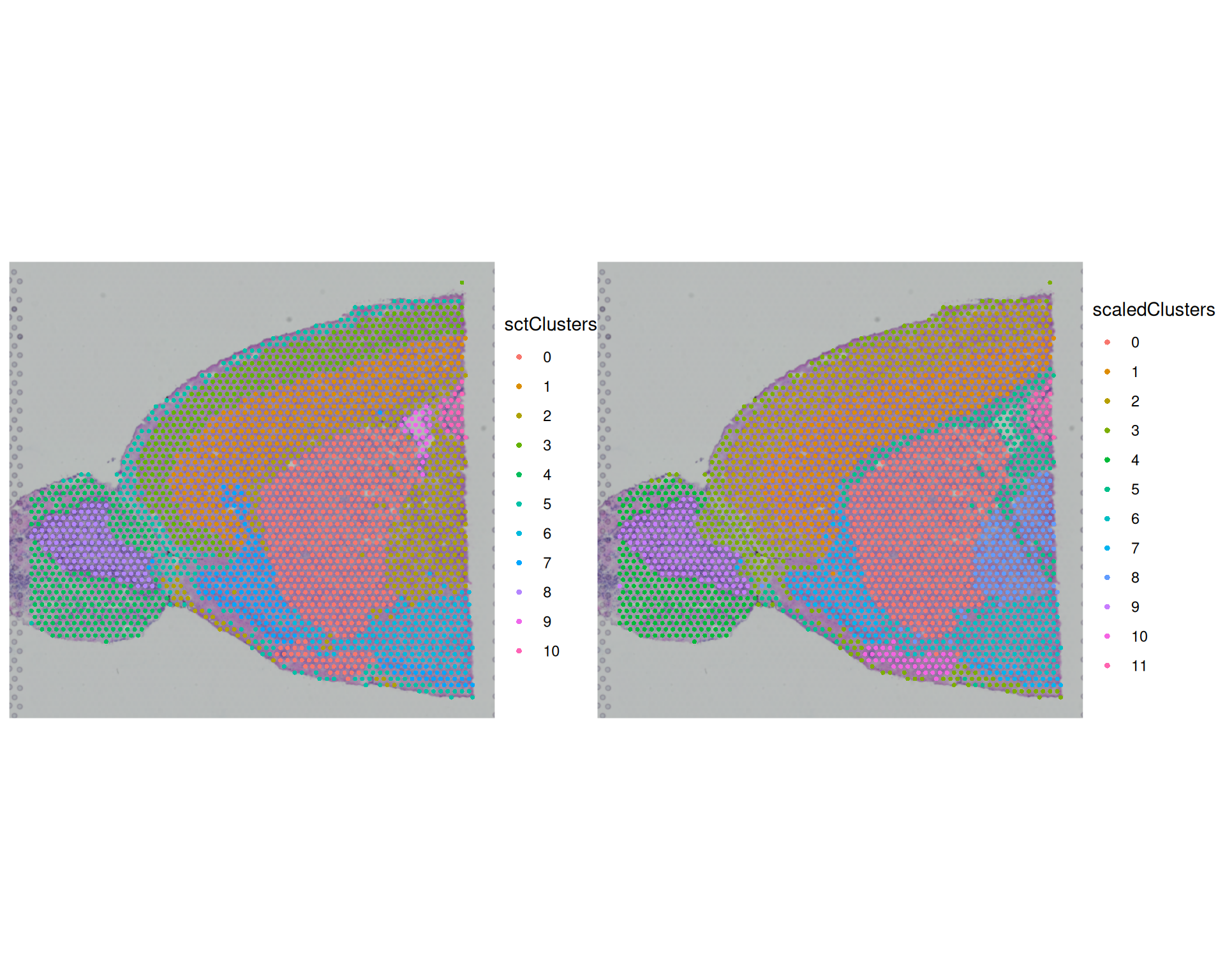
AAACATTTCCCGGATT-1 2.1070471 7 6We can use the SpatialDimPlot() function to visualise the clustering results for these methods:
SpatialDimPlot(
  visium,
  group.by = c("sctClusters", "scaledClusters"),
  ncol = 2
)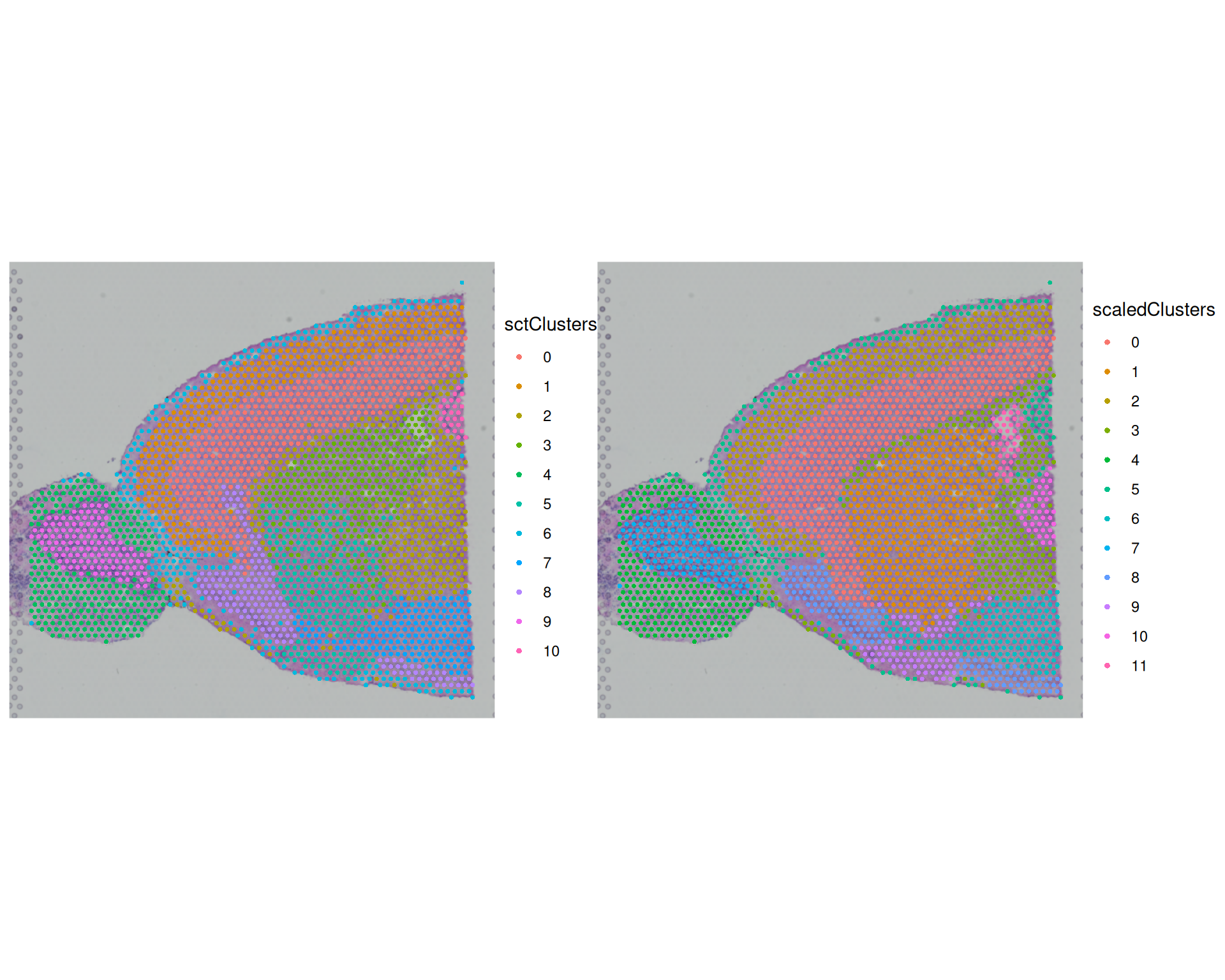
The broad spatial patterns are similar between methods, and several regions align with known anatomy (for example cortex and olfactory bulb). However, cluster boundaries and granularity differ. This shows that normalisation choice can change downstream structure, even when global patterns remain similar.
We can also quantify agreement using the Adjusted Rand Index (ARI) between clusterings. ARI compares whether pairs of spots are grouped together or apart in two solutions. An ARI of 1 indicates identical assignments; an ARI near 0 indicates chance-level agreement.
Use mclust::adjustedRandIndex() to compute ARI values:
# for adjustedRandIndex function
library(mclust)

# Calculate ARI between the two clusterings
adjustedRandIndex(visium$sctClusters, visium$scaledClusters)
[1] 0.7517838The ARI value between these two methods is quite high, indicating agreement between the methods.
6.9 Exporting the Normalised Data
After major analysis steps, save your Seurat object so you can restart your analysis without recomputing. At this stage the object contains several assays and layers, which increases memory use. If you plan to continue with one representation (for example SCT), you can remove unused assays or layers before saving.
# make SCT default assay
DefaultAssay(visium) <- "SCT"

# from "Spatial" assay keep the raw counts but remove the data and scale.data layers
visium[["Spatial"]]$data <- NULL
visium[["Spatial"]]$scale.data <- NULL
# save the Seurat object
saveRDS(visium, file = "results/mouse_brain_normalised_cleaned.rds")6.10 Exercises
ExerciseExercise 1 - Effect of Z-score transformation and mitochondrial regression
In the previous sections, we used workflows that regressed mitochondrial percentage and, where applicable, applied Z-score scaling with ScaleData().
Now repeat the analysis without mitochondrial regression and without Z-score scaling.
First, load the original filtered object into a new variable so you do not overwrite earlier results:
# Load the original filtered object
visium2 <- readRDS("precomputed/mouse_brain_filtered.rds")- Apply the SCTransform normalisation without regressing out mitochondrial percentage.
- Use the
NormalizeData()+ScaleData()functions for library size normalisation. Do not regress out mitochondrial percentage and do not transform the data into Z-scores. - Visualise the resulting clusters in a spatial plot and compare them with the earlier results.
AnswerAnswer
- SCTransform without mitochondrial regression:
# Apply SCTransform without regressing out mitochondrial percentage
visium2 <- SCTransform(
  visium2,
  assay = "Spatial"
)

# Confirm the new assay and layers
Layers(visium2[["SCT"]])
[1] "counts" "data" "scale.data"- Library size normalisation without scaling or mitochondrial regression:
# Perform log-normalisation without scaling or mitochondrial regression
visium2 <- visium2 |>
  NormalizeData(assay = "Spatial") |>
  ScaleData(assay = "Spatial", do.scale = FALSE, do.center = FALSE)

# Confirm the new layers
Layers(visium2[["Spatial"]])
[1] "counts" "data" "scale.data"- To visualise each normalisation result, first cluster the spots.
SpatialPlot()needs a grouping variable, so we run the same clustering workflow separately for each assay.
# SCTransform clustering
DefaultAssay(visium2) <- "SCT"
visium2 <- visium2 |>
  RunPCA() |>
  FindNeighbors(dims = 1:30) |>
  FindClusters(resolution = 0.5, cluster.name = "sctClusters")

# Library size normalisation clustering
DefaultAssay(visium2) <- "Spatial"
visium2 <- visium2 |>
  FindVariableFeatures() |>
  RunPCA() |>
  FindNeighbors(dims = 1:30) |>
  FindClusters(resolution = 0.5, cluster.name = "scaledClusters")

# Visualise
SpatialPlot(
  visium2,
  group.by = c("sctClusters", "scaledClusters"),
  ncol = 2
)
You can also compare the two clustering results with ARI:
# Calculate ARI between the different clusterings
adjustedRandIndex(visium2$sctClusters, visium2$scaledClusters)
[1] 0.8383366As before, the cluster agreement between the two methods is very high >0.8. Visually, the clusters also appear to have similar boundaries across the tissue.
We can also compare each method with and without mitochondrial regression to assess the effect of this choice directly.
# create a data frame to store the ARI results for each pair of clusterings
ari_results_mt_vs_no_mt <- data.frame(
  Method = c("SCTransform", "Scaled"),
  ARI = NA
)

# Calculate ARI between clusters with and without mitochondrial regression for each method
ari_results_mt_vs_no_mt$ARI[1] <- adjustedRandIndex(
  visium$sctClusters,
  visium2$sctClusters
)

ari_results_mt_vs_no_mt$ARI[2] <- adjustedRandIndex(
  visium$scaledClusters,
  visium2$scaledClusters
)

# view the ARI results
ari_results_mt_vs_no_mt
Method ARI
1 SCTransform 0.8565978
2 Scaled 0.8249880In this datest, it seems that regressing out the mitochondrial fraction did not have a big impact on the clusterings, as ARI is again very high at >0.8.
There is still no single “correct” result, and results may vary depending on the normalisation choices. We recommend looking at the scran normalisation in the extended materials for further discussion on this.
At the end of your exploration of normalisation methods, choose one that yields patterns consistent with known biology. Later, you can test robustness by repeating key downstream steps with at least one alternative normalisation.
6.11 Summary
TipKey Points
- Normalisation corrects for technical sources of variation that can hide biological signal.
- Library size (total reads per spot) is the primary confounder: spots sequenced more deeply appear to have higher expression for most genes.
- Other confounders, such as high mitochondrial fraction, can further affect expression profiles.
- Without normalisation, clustering can reflect technical artefacts rather than true tissue structure.
- Several normalisation approaches can be applied. We covered two:
SCTransform()fits a negative binomial model and applies variance stabilisation; usevars.to.regressto regress out confounders.NormalizeData()divides counts by library size and log-transforms; follow withScaleData()to Z-score and regress confounders.
- After normalisation, Seurat stores results in named layers within each assay; downstream steps such as PCA and clustering use
scale.databy default.counts: raw or model-corrected counts.data: log-transformed values used e.g. for visualisation.scale.data: Z-scored or sctransform residuals used for dimensionality reduction and clustering.
- Normalisation choice can affect downstream clustering results. Using spatial plots and the Adjusted Rand Index (ARI) can help in comparing methods.
- ARI values near 1 indicate near-identical cluster assignments; values near 0 indicate chance-level agreement.
- Even when ARI is high, spatial plots can reveal differences in cluster granularity and boundary location.
- No single normalisation method is universally optimal.
- Which method to choose can be informed by benchmarking studies and knowledge of tissue anatomy.
- A practical approach is to run multiple methods and confirm that biological conclusions are consistent across them.