8 Association tests and p-values
Caution
These materials are still under development
TipLearning objectives
- Summarise the statistical methods used by PLINK to carry out trait-genotype association tests.
- Interpret the effect sizes of an association in relation to individual genotypes.
- Distinguish how the interpretation of effect sizes differs for quantitative and binary trait models.
- Recognise the expected properties of p-values from association tests and how to troubleshoot potential biases.
- Explain the need to define genome-wide thresholds of significance.
8.1 Regression models
At its simplest, the association test carried out by software such as PLINK is based on linear regression models. Most GWAS software support two types of regression models, depending on the nature of the trait: normal regression for quantitative traits or binomial (logistic) regression for binary traits (case/control, yes/no, presence/absence).
We go over the intuition for each of these approaches. In the examples below we assume there are two alleles at a variant (i.e. it is bi-allelic), with alleles “A” and “B”. The three diploid genotypes are written as “AA”, “AB” and “BB”.
8.2 Quantitative trait models
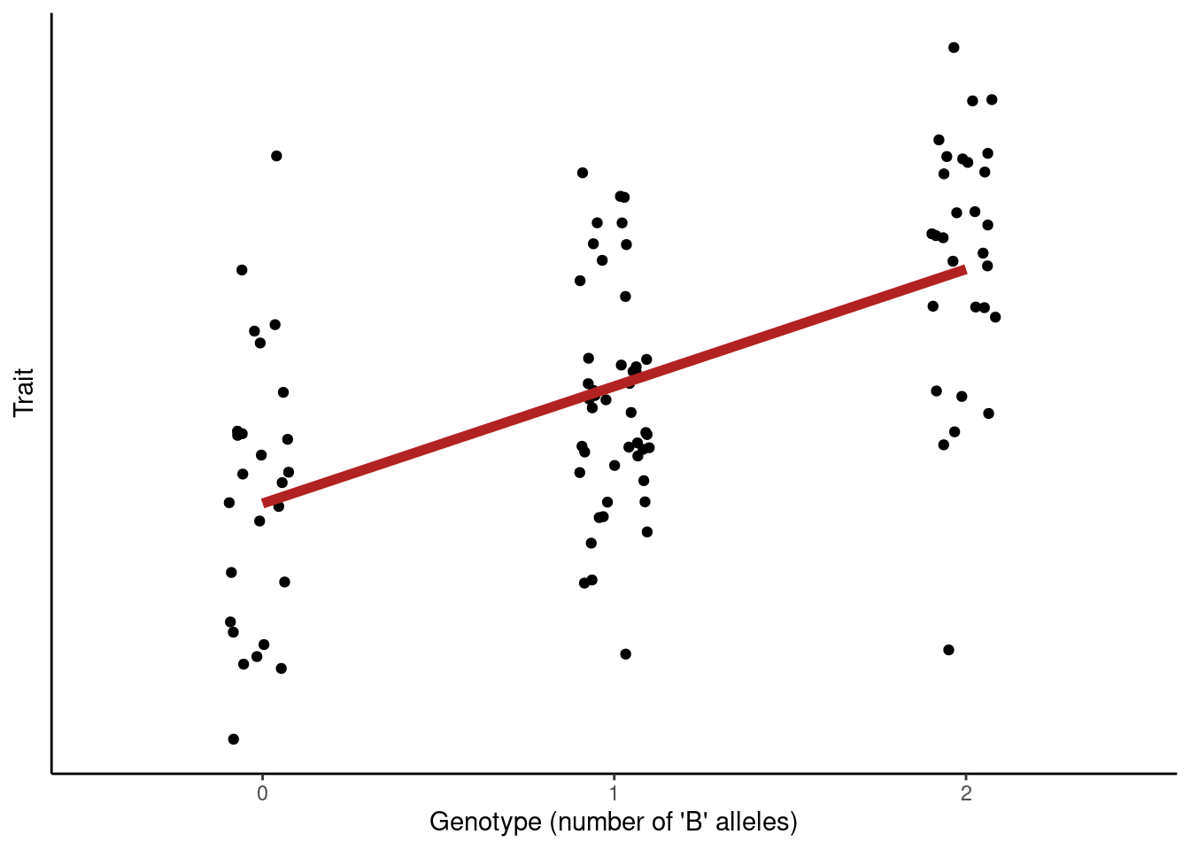
For quantitative traits we assume that the trait is well-approximated by a Normal distribution, \(Trait \sim N(\mu, \sigma^2)\) with mean \(\mu\) and variance \(\sigma^2\). The mean of this distribution is modelled as dependent on genotype, and we test for the significance of this relationship.
The strength of the relationship between genotype and trait is measured by the slope of the regression line, often referred to as Beta (β).
For example, if our trait was blood pressure measured in mm Hg, and we estimated β = 3 for a given variant, this would be the interpretation of the results:
- Genotype AA: baseline group (carrying zero “B” alleles).
- Genotype AB: +3 mg Hg compared to AA.
- Genotype BB: +6 mg Hg compared to AA.
This is a so-called “additive genetic model”, where we code the genotypes as “number of B alleles” and we thus assume that homozygotes “BB” increase by twice relative to heterozygotes.
The significance of association is determined by testing for the slope of the regression being zero (i.e. a flat line). This is done by using a t-statistic, which measures the “signal-to-noise” ratio of our estimate, and comparing it to a theoretical distribution to obtain a p-value for the association.
NoteQuantitative traits
Quantitative traits may include both continuous data (e.g. bmi, height) as well as discrete count data (e.g. cell count, cigarette consumption).
With generalised linear models, count data would usually be modelled using a more appropriate distribution rather than the Normal (e.g. a Poisson or Negative Binomial regression). However, these methods can be computationally expensive and so, in practice, software packages for GWAS usually only implement the normal regression model for quantitative traits. Additionally, GWAS sample sizes tend to be large (in the hundreds, thousands, or even millions), and so the normal approximation is a reasonable assumption even for discrete count variables.
8.3 Binary trait models
Conceptually, things are very similar for binary traits, except we assume the trait comes from a binomial (think of coin flips 🪙): \(Trait \sim Binomial(n, p)\) with known sample size \(n\) (that’s how many individuals we have) and a probability \(p\) that the event happens. The probability \(p\) is modelled as depending on genotype, and we test for the significance of this relationship.
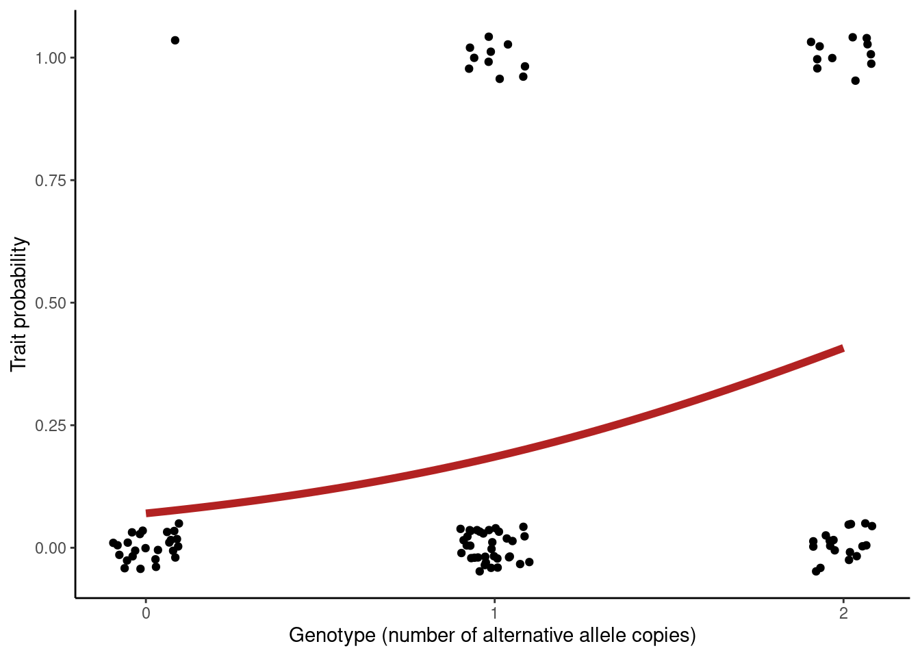
For binary traits, the strength of the relationship between trait and genotype is expressed as an odds ratio (OR), which compares the odds that the event happens in one group versus another. Let’s break this down. First, we define the odds of an event, which is the probability that the event occurs over the probability that it doesn’t:
\[ \text{Odds} = \frac{p}{1 - p} \]
Taking a concrete example, if our trait is “type 2 diabetes”, the odds represents the probability change in having this condition, relative to not having it:
\[ \text{Odds} = \frac{\text{probability diabetes}}{\text{probability healthy}} \]
An odds ratio is then the ratio of odds between two groups. In the context of GWAS, we report odds ratios per-allele increase, i.e. between a group that has 1 allele versus the group without that allele. Taking our T2D example and assuming the “AA” genotype is our reference group, then the odds ratio would be:
\[ \text{Odds Ratio} = \frac{\text{odds diabetes for genotype AB}}{\text{odds diabetes for genotype AA}} \]
One important thing to consider is that odds ratios are multiplicative. For example, if the estimate for a given variant was OR = 3 per allele, the interpretation in terms of genotypes is:
- Genotype AA: baseline group (carrying zero “B” alleles).
- Genotype AB: 3 times more likely to have the condition than AA.
- Genotype BB: 3² = 9 times more likely to have the condition than AA.
The significance of association in this case is assessed using a Wald Z-statistic, which similarly to the t-statistic discussed earlier, measures the “signal-to-noise” ratio of our OR estimate. As usual, this is compared to a theoretical distribution to obtain a p-value for the association.
ImportantEffect sizes
In the examples given above we used relatively large effect sizes, for illustration purposes. For complex traits the effects of individual variants might be quite small. For example, for type 2 diabetes many found associations have OR of ~1.1 or even less. For reference, this represents a probability of 52% of having the disease compared to 48% for not having it.
These are still substantial effects, but not as large as what we used in the examples above.
NoteOdds ratios, odds, log-odds and probabilities (click to learn more)
Logistic regression models can be challenging to interpret and working with odds is sometimes confusing. Remember, the odds is a ratio of two probabilities: the probability of an event happening versus it not happening.
Because of the underlying maths, logistic regression coefficients are usually given as log-odds. This is exactly how it sounds like, it’s the natural log of the odds ratio, also known as the logit function. This transformation is useful as it converts odds, which range from 0 to infinity, to a range of \((-\infty, +\infty)\), which is easier to work with for the underlying statistical machinery.
I can be useful to convert probabilities to odds (or log-odds) and back. Say an event has a 75% chance of happening, meaning the odds are 3:1. We can calculate the odds and log-odds like so:
# if you know your probability
probability <- 0.75

# calculate odds as:
odds <- probability / (1 - probability)
odds
[1] 3# and log-odds taking the natural log of the previous
log_odds <- log(odds)
log_odds[1] 1.098612On the other hand, if you start from having the odds, for example odds = 3, then you need to: first convert it to log-odds (aka “logit”); then use the inverse-logit function to calculate the probability. Here’s the R code:
# if you know your odds
odds <- 3

# Inverse-logit: convert log-odds back to probability
probability <- plogis(log(odds))
probability
[1] 0.75Finally, if you have an odds ratio, you need to remember that this is the ratio of the odds of two groups, which is not the same as the ratio of their probabilities.
For example, if the baseline probability is 0.1, then the odds are 0.1/(1-0.1) = 0.1111. If the odds ratio is 3, then the odds of the second group are 3 times larger than the first group, i.e. 0.3333. If we convert this back to a probability (using the inverse-logit function shown above), we would get 0.25, which is not 3 times larger than the baseline probability of 0.1.
As we said, it can be confusing to work with odds, but it’s worth spending some time to let these ideas sink in if you work with binary data often.
8.4 P-value distribution
In addition to the genotype effect (β or OR), another output of the statistical association test is the p-value of the statistical test for its significance. The association test is performed separately for each variant, so we get as many p-value as there are variants. One of the first steps when analysing the outcome of an association test is to assess potential biases, which can be diagnosed by looking at the p-value distribution.
In statistical null hypothesis testing, there is a theoretical expectation that p-values follow a uniform distribution when no effect exists. A p-value of 0.01 is just as likely as a p-value of 0.99 - it’s all just due to random chance. In our case, this would mean no association between the trait and genotype.
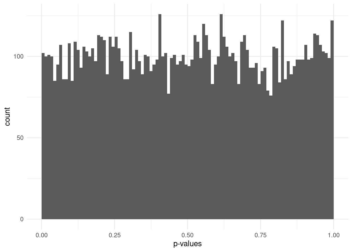
In a multiple testing scenario such as GWAS, where many tests being performed (one per variant), we would expect that most variants follow this uniform distribution.
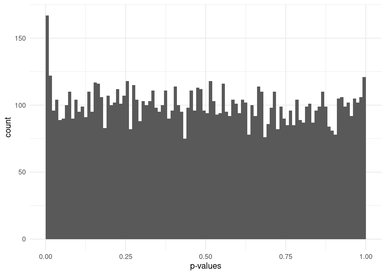
However, if some fraction of the variants are associated with the trait, this will skew the p-value distribution, leading to an excess of small p-values.
There is an excellent post in the Variance Explained blog, with further discussions on this topic: How to interpret a p-value histogram, by David Robinson.
8.4.1 Q-Q plots
Another way to assess the distribution of p-values is to produce a Q-Q plot, which is a type of scatterplot that compares the distribution of p-values under the expected uniform distribution and the actual observed p-values.
For Q-Q plots it is common to plot the p-values as \(-log_{10}(p-value)\), which is a transformation that emphasises very small p-values. As small p-values is what we expect to see for “significant” associations (and is what we’re ultimately hoping to see!), this emphasises those very small values by transforming them into relatively large numbers.
Here are the Q-Q plots of the expected-versus-observed \(-log_{10}(p-value)\) for each of the distributions shown above:
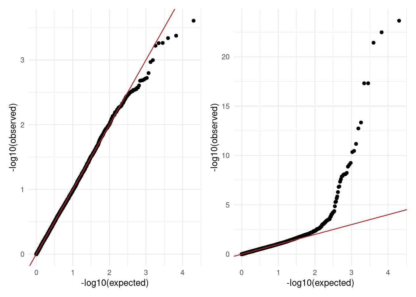
The diagonal line indicates the expectation under the null hypothesis. As we can see in the examples above, the plot on the left shows all points falling along the diagonal, indicating no significant associations. The plot on the right, on the other hand, shows good fit for part of the distribution, but with an excess of small p-values as shown by a deviation of points towards the top of the graph.
8.5 Summary
TipKey Points
- The statistical methods used for association analysis are based on linear regression models.
- Quantitative traits are analysed using normal linear regression, whereas binary traits are modelled using binomial (logistic) regression.
- The effect sizes of quantitative traits are reported as unit increase per allele and can be interpreted linearly.
- The effect sizes of binary traits are reported as odds ratios per allele and are multiplicative.
- In a multiple testing setting, p-values are expected to follow a uniform distribution under the null hypothesis.
- In general, the distribution of the observed p-values should follow the uniform expectation, except for a few variants that are associated with the trait.
- Q-Q plots can be used to assess the expected versus observed p-value distributions.
- Large deviations from expectation may indicate biases in the analysis that lead to p-value inflation.
- Due to multiple testing, a stringent p-value threshold is needed.
- For human GWAS p-value thresholds have been determined based on the general LD patterns observed across the human genome.