# load the libraries
library(tidyverse) # data manipulation
library(patchwork) # to compose plots
library(janitor)   # to clean column names
theme_set(theme_minimal()) # change default ggplot2 theme6 Sample QC
Caution
These materials are still under development
TipLearning objectives
- List metrics that can be used for sample-level quality control and filtering.
- Use PLINK to calculate genotype call rates, heterozygosity, discordant sex and sample relatedness.
- Analyse quality metric results in R and assess the need for filtering in downstream analyses.
- Discuss how these quality metrics are impacted by population structure.
6.1 Per-sample metrics
Similarly to what we did for variants, we also investigate quality issues in our samples. We will consider the following metrics for each sample:
- Call rate: Fraction of missing genotypes. Variants with a high fraction of missing data may indicate overall low quality for that sample and thus be removed from downstream analysis.
- Heterozygosity: The fraction of SNVs that are heterozygous in a given sample. We expect most individuals to have a mixture of both homozygous and heterozygous SNVs. Outliers may indicate genotyping errors.
- Relatedness: Individuals who are related to each other (e.g. siblings, cousins, parents and children) may affect the association test results and create false positive hits. It is therefore good to assess if there are potential close family members before proceeding.
- Discordant sex: In humans, we expect males to have only one X chromosome and thus no heterozygous variants, while the converse is true for females. This expectation can be used to identify potential mis-matches and correct them before proceeding.
We will cover each of these below.
ImportantSet up your R session
If you haven’t done so already, start an R session with the following packages loaded:
6.2 Call rates
Similarly to what we did for variants, we can calculate how many missing genotypes each individual sample has. This can then be used to assess the need to exclude samples from downstream analyses.
There are no set rules as to what constitutes a “good call rate”, but typically we may exclude samples with greater than ~5% of missing genotypes. This threshold may vary, however, depending on the nature of data you have.
As we saw before, the option --missing generates missingness files for both samples and variants, so we don’t need to re-run the PLINK command. However, here it is as a reminder:
plink2 \
  --pfile data/plink/1000G_subset \
  --out results/1000G_subset \
  --missing
For the sample missingness report the file extension is .smiss, which we can import into R as usual:
smiss <- read_tsv("results/1000G_subset.smiss") |>
  clean_names(replace = c("#" = ""))

# inspect the table
head(smiss)
# A tibble: 6 × 6
iid super_pop population missing_ct obs_ct f_miss
<chr> <chr> <chr> <dbl> <dbl> <dbl>
1 HG00097 N N 0 4467560 0
2 HG00107 N N 104 4474704 0.0000232
3 HG00108 N N 96 4474704 0.0000215
4 HG00109 N N 35707 4474704 0.00798
5 HG00110 N N 0 4467560 0
6 HG00111 N N 0 4467560 0 We can tabulate how many samples have missing genotypes:
table(smiss$missing_ct > 0)
FALSE  TRUE
  408   629
Around 61% of our samples have missing data in at least one of the variants.
For those samples with some missing data, we can check the distribution of the fraction of missing genotypes:
smiss |>
  filter(f_miss > 0) |>
  ggplot(aes(f_miss)) +
  geom_histogram()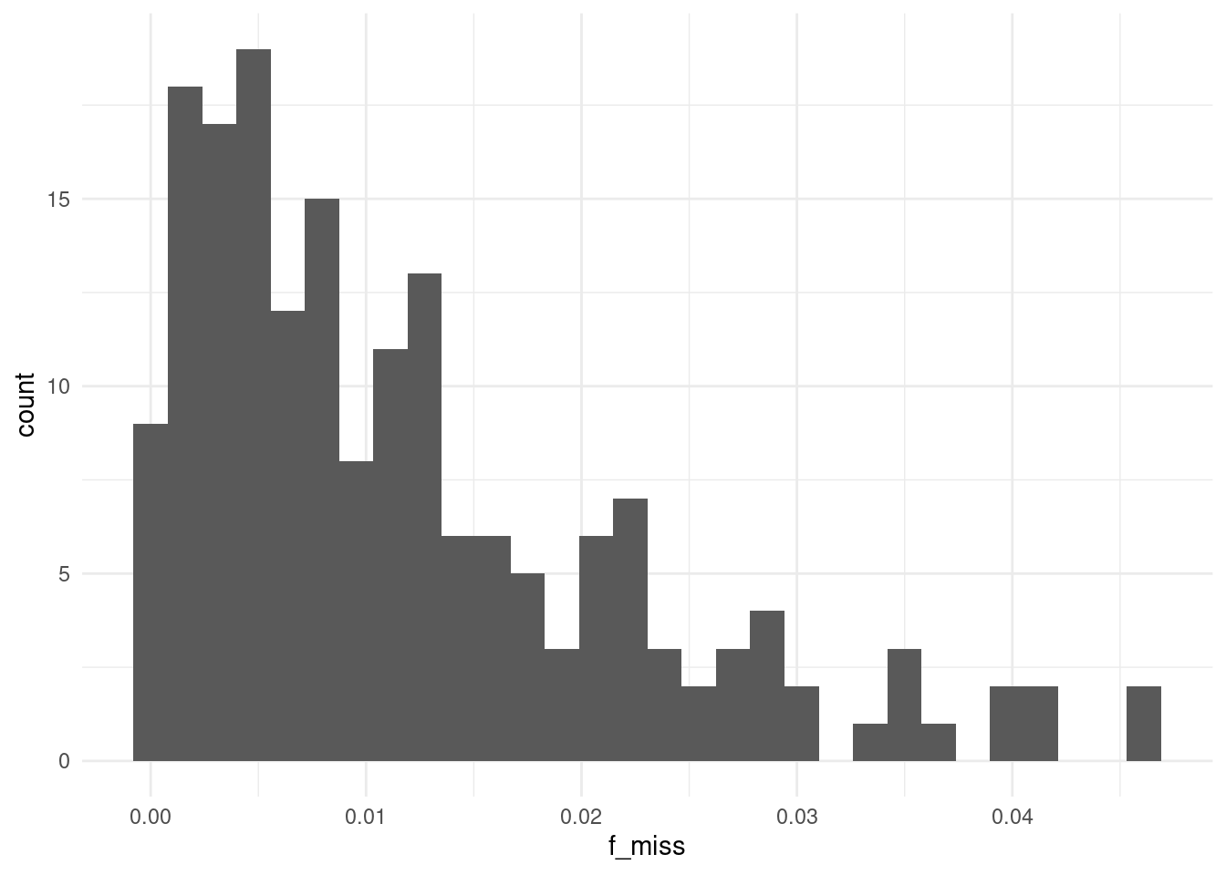
From this distribution it seems that most individuals have a low fraction of missing genotypes, indicating no problematic samples.
A filter is probably not even necessary in this case, as no sample seems to have more than 5% missing data. In any case, individuals with high rates of missing data, e.g. using the 5% threshold, can be excluded using PLINK’s option --mind 0.05.
6.3 Heterozygosity and inbreeding
Another useful metric to assess issues with sample quality is to look at the fraction of variants that are heterozygous, or conversely what the inbreeding coefficient of each individual is. In general, we expect an individual to have both homozygous and heterozygous genotypes. Individuals with high heterozygosity may represent poor quality samples (e.g. contaminated samples composed of a mixture of DNA from two individuals). Conversely, individuals with high homozygosity may indicate inbreeding, which can impact the balance of allele frequencies in the population (as discussed in the Hardy-Weinberg equilibrium section) and potentially bias the results of our association tests.
There isn’t necessarily a clear value, but within a population we should expect the distribution of heterozygosity to be consistent across individuals. If an individual is an outlier (e.g. with too many homozygous or heterozygous sites), then we may infer some quality issues may have ocurred with that sample.
PLINK can calculate per-sample heterozygosity rates using the option --het:
plink2 \
  --pfile data/plink/1000G_subset \
  --out results/1000G_subset \
  --extract results/1000G_subset.prune.in \
  --geno 0.05 --maf 0.01 --mind 0.05 \
  --het
In this command we also apply the variant filters defined in the variant QC section. Namely, retaining genotypes and samples with a call rate of at least 95% (--geno 0.05 --mind 0.05) and minor allele frequency of at least 1% (--maf 0.01). And use the --extract option to only include uncorrelated variants, obtained by LD prunning.
The output file has extension .het, which we can import into R:
het <- read_tsv("results/1000G_subset.het") |>
  clean_names(replace = c("#" = ""))

head(het)
# A tibble: 6 × 5
iid o_hom e_hom obs_ct f
<chr> <dbl> <dbl> <dbl> <dbl>
1 HG00097 511803 494932 602310 0.157
2 HG00107 509813 494932 602310 0.139
3 HG00108 510716 494932 602310 0.147
4 HG00109 504334 490975 597513 0.125
5 HG00110 513805 494932 602310 0.176
6 HG00111 511396 494932 602310 0.153We have four values for each individual:
o_homis the number of observed homozygous genotypes.e_homis the expected number of homozygous genotypes, based on the allele frequencies in the population and under Hardy-Weinberg equilibrium (HWE).obs_ctis the number of non-missing genotypes.fis the inbreeding coefficient, which represent the individual heterozygosity relative to the expectation under HWE (see box below for details on its calculation).
NoteInbreeding coefficient calculation
Let’s call \(H_{obs}\) the observed fraction of heterozygote variants in an individual and \(H_{exp}\) the expected heterozygosity under Hardy-Weinberg equilibrium (HWE).
The inbreeding coefficient is usually defined as:
\[ F = 1 - \frac{H_{obs}}{H_{exp}} \]
I.e., it is the difference between the expected and observed heterozygosity, divided by the expected heterozygosity.
- A value of 0 would indicate that the individual is heterozygous at the expected rate, since \(H_{obs} = H_{exp}\).
- A value of 1 would indicate that the individual is completely homozygous, since \(H_{obs} = 0\).
- If \(H_{obs} < H_{exp}\), then the inbreeding coefficient will be between 0 and 1, indicating different levels of homozygosity or inbreeding.
- If \(H_{obs} > H_{exp}\), then the individual is more heterozygous than expected under HWE and the inbreeding coefficient takes negative values.
Rather than reporting the observed and expected heterozygosity, PLINK reports things as counts of homozygous variants. Because all of these can be calculated from each other, we can rearrange the equation above to express the inbreeding coefficient in terms of the number of homozygous genotypes.
Let’s call \(O_{hom}\) the number of observed homozygous genotypes, \(E_{exp}\) the number of expected homozygous genotypes and \(O_{total}\) the total number of variants. Then, the equation above could be written as:
\[ F = 1 - \frac{O_{total} - O_{hom}}{O_{total} - E_{hom}} \]
Which we can further rearrange to:
\[ F = \frac{O_{hom} - E_{hom}}{O_{total} - E_{hom}} \]
We can confirm this is how PLINK calculates the inbreeding value:
het |>
  mutate(f2 = (o_hom - e_hom) / (obs_ct - e_hom))
# A tibble: 1,037 × 6
iid o_hom e_hom obs_ct f f2
<chr> <dbl> <dbl> <dbl> <dbl> <dbl>
1 HG00097 511803 494932 602310 0.157 0.157
2 HG00107 509813 494932 602310 0.139 0.139
3 HG00108 510716 494932 602310 0.147 0.147
4 HG00109 504334 490975 597513 0.125 0.125
5 HG00110 513805 494932 602310 0.176 0.176
6 HG00111 511396 494932 602310 0.153 0.153
7 HG00112 504590 488807 594863 0.149 0.149
8 HG00114 510423 494932 602310 0.144 0.144
9 HG00118 508905 494932 602310 0.130 0.130
10 HG00119 511823 494932 602310 0.157 0.157
# ℹ 1,027 more rowsLet’s consider the distribution of inbreeding coefficients for the individuals in our sample. A value of 0 indicates that the individual is heterozygous at the expected rate, while a value of 1 indicates that the individual is completely homozygous. Negative values indicate that the individual is more heterozygous than expected under HWE.
We can make a histogram of the inbreeding coefficient:
het |>
  ggplot(aes(f)) +
  geom_histogram()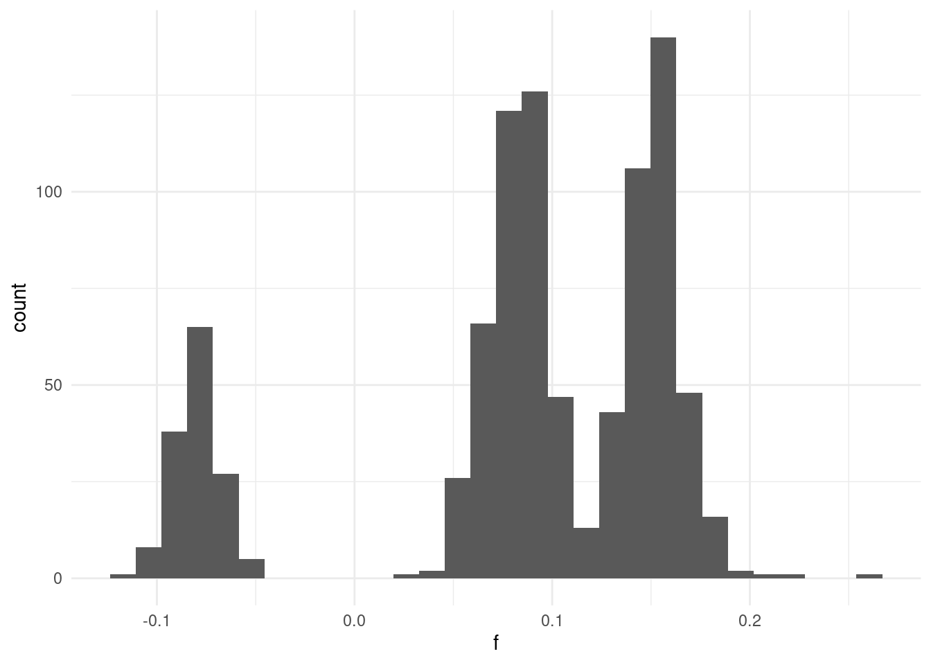
In general we can see there are no individuals with very extreme inbreeding values (e.g. close to 1). We can see some individuals with slightly negative values, indicating they are more heterozygous than expected under HWE.
The main issue we see is that the distribution is multi-modal. This indicates that we have different groups of samples, some with higher rates of inbreeding and others with lower rates.
This is likely a consequence of the fact we have individuals from different populations (geographic areas). This is an issue we will come back to in the population structure chapter.
For now, it is clear that we cannot easily filter samples based on their heterozygosity, as the populations are heterogeneous.
6.4 Sample relatedness
One other thing that can be considered is whether there are potential relationships within your samples. In our dataset all samples are supposed to be unrelated.
plink2 \
  --pfile data/plink/1000G_subset \
  --out results/1000G_subset \
  --extract results/1000G_subset.prune.in \
  --geno 0.05 --maf 0.01 --mind 0.05 \
  --make-king-table
This outputs a file with format .kin0, which contains pairwise kinship coefficients for each pair of samples. We can read this table into R as usual:
king <- read_tsv("results/1000G_subset.kin0") |>
  clean_names(replace = c("#" = ""))

head(king)
# A tibble: 6 × 6
iid1 iid2 nsnp hethet ibs0 kinship
<chr> <chr> <dbl> <dbl> <dbl> <dbl>
1 HG00107 HG00097 602310 0.0543 0.0271 -0.00541
2 HG00108 HG00097 602310 0.0533 0.0267 -0.00315
3 HG00108 HG00107 602310 0.0552 0.0260 0.00805
4 HG00109 HG00097 597513 0.0560 0.0268 -0.00131
5 HG00109 HG00107 597513 0.0568 0.0256 0.0145
6 HG00109 HG00108 597513 0.0563 0.0260 0.00769For each pair of samples we now have the kinship coefficient calculated using the KING method. The authors of this method indicate that unrelated individuals should have a kinship coefficient of zero, but they recommend using a threshold of ~0.044 (cf. Table 1 in Manichaikul et al. 2010).
We can check how many individuals are above this threshold:
table(king$kinship > 0.044)
 FALSE   TRUE
537152     14
Only 14 individuals are above this threshold. We can also look at the distribution of this kinship coefficient:
king |>
  ggplot(aes(kinship)) +
  geom_histogram(bins = 100) +
  geom_vline(xintercept = 1/16)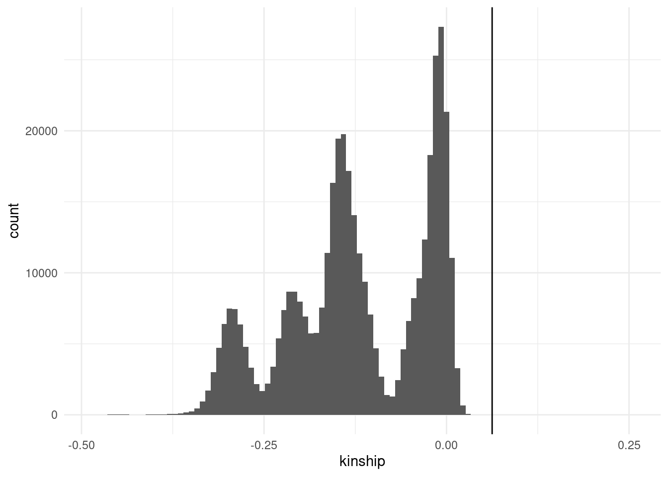
Similar to what we’ve seen before for heterozygosity, we get a multi-modal distribution of kinship values. This is again likely because of population structure, i.e. the fact that our samples come from different geographic areas and thus may have differing base levels of “residual relatedness”.
However, we can see all most values are negative, which can happen with this coefficient and essentially indicates no relatedness between individuals.
More worringly, we can see some individuals seem closely related if we sort the table in descending order of kinship and look at the top few rows:
king |>
  arrange(desc(kinship)) |>
  head(n = 15)
# A tibble: 15 × 6
iid1 iid2 nsnp hethet ibs0 kinship
<chr> <chr> <dbl> <dbl> <dbl> <dbl>
1 HG00581 HG00578 600692 0.0861 0.00503 0.266
2 HG00635 HG00578 592174 0.0832 0.00564 0.252
3 NA20900 NA20882 596183 0.0787 0.000112 0.251
4 HG00635 HG00581 590772 0.0789 0.00680 0.232
5 NA19664 NA19660 602310 0.0648 0.0162 0.0998
6 HG03457 HG03454 602310 0.0750 0.0229 0.0731
7 NA19312 NA19307 598342 0.0752 0.0232 0.0713
8 HG03372 HG03301 602310 0.0744 0.0232 0.0705
9 HG00607 HG00578 596988 0.0575 0.0187 0.0682
10 HG03998 HG03866 600897 0.0620 0.0201 0.0661
11 NA19384 NA19025 602310 0.0728 0.0238 0.0626
12 HG00595 HG00577 602310 0.0569 0.0201 0.0558
13 HG00607 HG00581 595469 0.0553 0.0199 0.0538
14 HG00635 HG00607 587561 0.0550 0.0198 0.0526
15 NA20346 NA20340 591675 0.0709 0.0264 0.0432We see a few individuals have a kinship coefficient of ~1/4, which is indicative of full siblings. Others are close to ~1/8 (second degree relationships, e.g. cousins) and a few close to ~1/16 (third degree relationship).
To eliminate close relationships from downstream analysis, we can use PLINK’s option --king-cutoff 0.125 to eliminate at least second degree relationships.
6.5 Discordant sex
CautionWork in progress
Sorry, this section isn’t yet finished. There’s a brief explanation below, but we are still working on having data suitable to demonstrate this analysis.
Another thing that can be checked is whether the sex assigned to each of our samples is correct, based on the genetic data. This relies on having genotypes in a sex chromosome and checking whether the heterozygosity matches the expectation. For example, in humans males have one copy of the X chromosome, and females two. Therefore, all males should be homozygous for variants in the X chromosome, whereas females may have a mixture of heterozygous and homozygous sites.
We can do this quality check using PLINK’s --check-sex option:
plink2 --pfile data/plink/1000G_subset --out results/1000G_subset --check-sexUnfortunately this does now work in our example data, as we are missing genotypes on the X chromosome.
6.6 Summary
TipKey Points
- Key metrics for sample-level quality control include: call rate, heterozygosity, relatedness and sex assignment.
- Call rates (
--missing): samples with low call rates (e.g. <95% or >5% missing genotypes) are typically excluded.- To remove samples missing genotypes above a certain threshold use
--mind X(replaceXwith the desired fraction, e.g. 0.05).
- To remove samples missing genotypes above a certain threshold use
- Heterozygosity (
--het): samples that are outlier with regards to the number of heterozygous variants relative to other samples are typically excluded as they may represent errors (e.g. mixed samples or genotyping errors).- It is common practice to remove samples a certain number of standard deviations away from the observed distribution (e.g. +/- 3 SDs).
- However, this should only be applied to samples from relatively homogenous populations, as different sub-populations may have different distributions.
- Sample relatedness (
--king): even when individuals are thought to be unrelated, there may be some criptic relatedness that was previously unknown. Excluding very close relatives is best-practice to avoid biasing downstream association tests.- To exlude individuals above a certain kinship score threshold use
--king-cutoff X(replaceXwith the desired threshold). Common thresholds include 1/4 for full siblings, 1/8 for second degree relatives and 1/16 for third degree relatives.
- To exlude individuals above a certain kinship score threshold use
- Discordant sex (
--check-sex): it is good practice to check if the sex assigned to the individual (specified in the.psam/.famfile) matches the sex from genetic data. This can be determined from genotypes in the sex chromosomes. Individual with discordant sex may either be corrected or removed from the analysis.