4  PLINK basics

Caution

These materials are still under development

Learning objectives

• Recognise how the PLINK software can be used for GWAS analysis.
• List the file formats required by PLINK.
• Recognise the general structure of a PLINK command and the structure of the output files it generates.
• Use R to import, explore and visualise the results generated by PLINK.

4.1 The PLINK software

The PLINK software provides an extensive toolkit for genome wide association analysis. Amongst its many functions, it includes:

• Calculation of basic statistics such as genotype counts, allele frequencies, missing data, measures of inbreeding, checking sex assignment.
• Measures of linkage disequilibrium between variants and genetic relatedness between samples.
• Assessment of population stratification using principal components analysis.
• Perform association tests using generalised linear models between genotypes and quantitative or binary traits.

PLINK has been designed to work with large data, being highly efficient and take advantage of multiple processors (CPUs) to run tasks in parallel.

It has excellent documentation, which goes into great details about its functions and both input and output file formats.

PLINK version 2 is still under active development and many of its functions have been updated from PLINK version 1 to deal with ever increasing amounts of data. While most of the functions have been ported from PLINK 1 to PLINK 2, some functionality may still be missing from the more recent version. We will use PLINK 2 throughout these materials, but it is worth being aware that some functions may only be available on the older version.

4.2 PLINK input files

PLINK requires three types of input files: genotypes, variant information and sample information. With version 2 of PLINK new file formats for these files were implemented, however PLINK 2 supports both the new and older file format versions.

Description	PLINK 1 Format	PLINK 2 Format
Genotypes stored in a binary (compressed) file format.	.bed	.pgen
Variant information file containing chromosome, position, reference, and alternative alleles for each variant.	.bim	.pvar
Sample information file specifying sample IDs, parents (if known), and sex (if known). Family IDs are used for related individuals, while they can be set to missing for unrelated individuals.	.fam	.psam

Don’t get your BED files confused

The .bed format used by PLINK 1 is distinct from the BED (Browser Extensible Data) format often used in bioinformatics to represent the coordinates of genomic features (e.g. genes).

These are completely different files, which unfortunately ended up being referred to by the same file extension. That is one reason why the newer PLINK 2 now uses the more distinct .pgen extension for its genotype file.

4.2.1 Example data

In these materials we use genotype data from the 1000 Genomes project, specifically the 30x data described in Byrska-Bishop et al. (2022). We have down-sampled the SNVs, to retain ~6M out of the ~70M available.

Variants calls are often stored as VCF (Variant Call Format) files (cf. the data on the 1000G server). PLINK allows us to convert VCF files into its required input formats using the --make-pgen (PLINK 2 format) or --make-bed (PLINK 1 format) options.

We already provide a set of .pgen/.bed, .pvar/.bim and .psam/.fam files based on the publicly-available data.

In addition to genotype data, we will use simulated traits, based on real GWAS results on quantitate and binary traits:

• Binary trait: type 2 diabetes , study accession GCST006801.
• Binary trait: chronotype (“morning person”), study accession GCST007565.
• Quantitative (continuous) trait: caffeine consumption (“mg/day”), study accession GCST001032.
• Quantitative (continuous) trait: blood pressure (mm Hg) study accession GCST001235

4.3 Working with plink

PLINK has many functions available, but we will start with a simple one that calculates allele frequencies for each of our variants:

plink2 --pfile data/plink/1000G_subset --out results/1000G_subset --freq

You can see the structure of the command is:

• plink: the name of the program.
• --pfile: input file name prefix. PLINK will then look for files with .pgen, .psam and .pvar extensions that all share the prefix specified here.
• --freq: option to calculate allele frequencies, detailed in the documentation.
• --out: output file name prefix. PLINK will generate all the output files with this common prefix and a file extension specific to each command. In this example we only get an allele frequency file (detailed below). You can omit this option, in which case PLINK will output the files to the same directory as specified with --pfile. However, it’s good practice to keep our results files separate from the original raw data.

Most PLINK analysis options output their results to a file with an extension that is specific to that option. In the example of the --freq option, it outputs a file with .afreq extension. This is detailed in the documentation of each option.

4.4 Analysing PLINK files in R

PLINK’s output files are standard text files, usually consisting of tables with tab-separated values (TSV). Therefore, they can be read and analysed in R (or Python, if you prefer).

Let’s start our analysis in R by loading some packages:

# load the libraries
library(tidyverse) # data manipulation
library(patchwork) # to compose plots
library(janitor)   # to clean column names
theme_set(theme_minimal()) # change default ggplot2 theme

We now read the .afreq file produced by the PLINK command we ran earlier:

# read the allele frequency file
afreq <- read_tsv("results/1000G_subset.afreq") |> 
  # PLINK's column names are always upppercase
  # this makes them lowercase, easier to type
  clean_names()

# inspect the file
head(afreq)

# A tibble: 6 × 6
  number_chrom id    ref   alt   alt_freqs obs_ct
         <dbl> <chr> <chr> <chr>     <dbl>  <dbl>
1            1 .     G     A       0.0775    1806
2            1 .     A     G       0.315     1806
3            1 .     A     T       0.00332   1806
4            1 .     T     G       0         1762
5            1 .     C     G       0.00443   1806
6            1 .     G     A       0.119     1806

We used the read_tsv() function, which imports tab-separated files as a data frame, followed by the clean_names() function (from the janitor package) to conveniently convert the column names to lowercase (it also removes spaces and other special characters, if present).

We can now use this data frame to produce a histogram of the allele frequencies in our population, using standard ggplot2 functions:

# plot a histogram of alternative allele frequencies
afreq |> 
  ggplot(aes(alt_freqs)) +
  geom_histogram(binwidth = 0.01)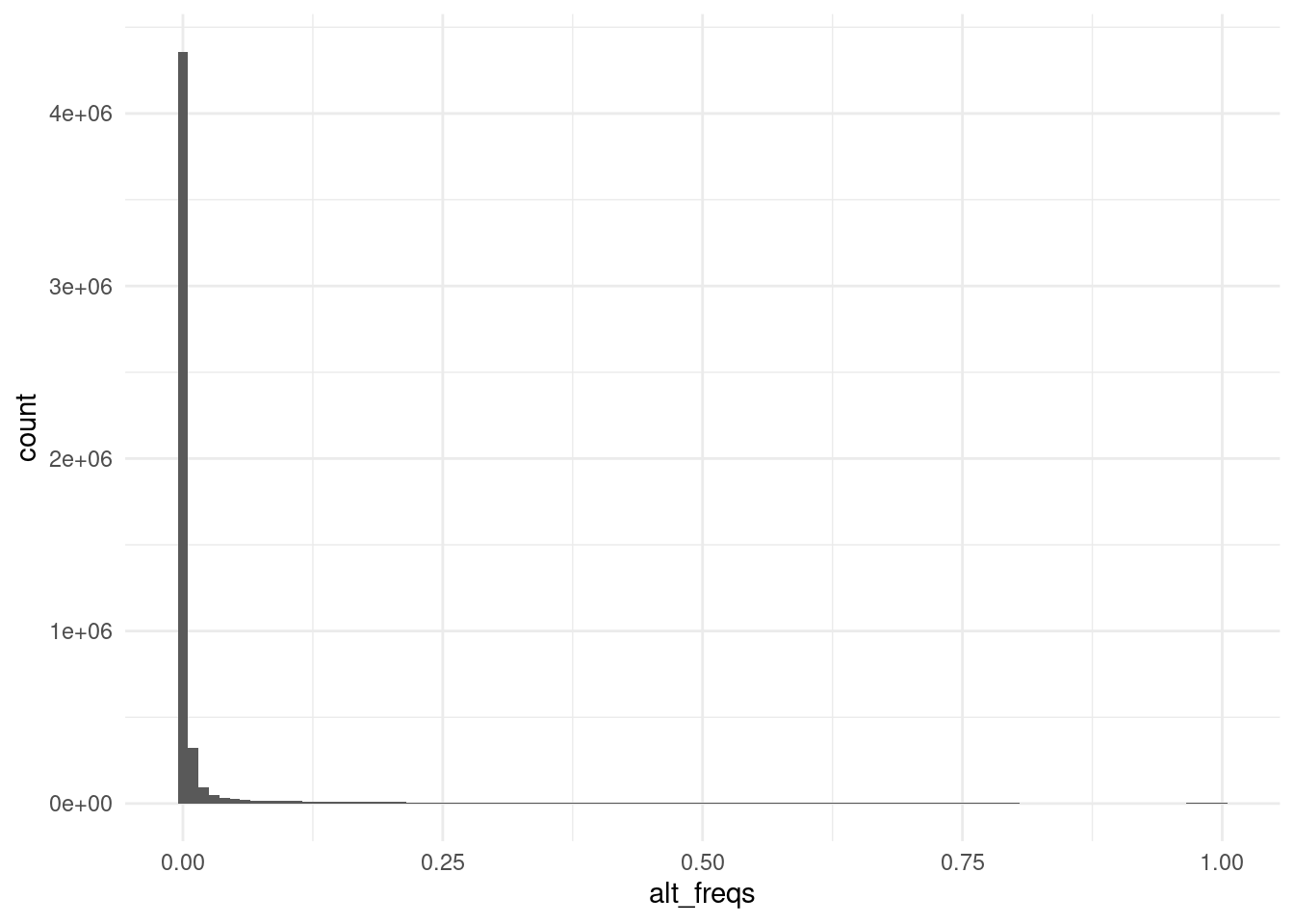

We can see many variants with a frequency close to zero for the alternative allele, indicating a high fraction of variants may be very rare or even not vary in this collection of samples. We will likely need to do some filtering before proceeding with our analysis, which is the topic of the next chapters.

4.5 Summary

Key Points

• PLINK is a widely-used software for GWAS, as it includes a wide range of functions, from quality control to downstream analysis.
• PLINK requires three critical types of input:
  • Genotype data (.pgen/.bed).
  • Information about genetic variants (.pvar/.bim).
  • Information about the samples (.psam/.fam).
• A typical PLINK command will include:
  • Option specifying the input files’ prefix: --pfile (or --bfile if using the older formats).
  • Option specifying the output files’ prefix: --out.
  • Other options specifying the task we want it to
• PLINK generates output files with specific extensions for each option it provides. All file extensions are detailed in the documentation.
• Most of PLINK’s output files are simple text files with tab-separated values (TSV), which can therefore be imported to standard data analysis software such as R.