library(tidyverse)
library(rstatix)

library(performance)
library(ggResidpanel)

library(MASS)

library(pwr)10 Power analysis
In this chapter, we’ll look at running a standard power analysis via simulation for some of the datasets you generated in earlier chapters, and compare this to standard functions.
Currently, this chapter is written only in R. Python code will be added at a later date.
10.1 Libraries and functions
NoteClick to expand
10.1.1 Libraries
10.2 A quick reminder/primer on statistical power
For this section, we’ll focus on the classic idea of statistical power: the probability of extracting a significant p-value from your dataset, given that the null hypothesis is false.
We typically perform power analysis “analytically” - of the following components:
- Desired power
- Significance level
- Estimated effect size
- Sample size
we can always calculate the fourth if we know the other three.
However, the analytical method has some major cons (in my opinion):
- It only works for linear models - this is a non-controversial downside!
- It gives a very “fixed” or static impression of things. For example, people rarely explore a range of estimated effect sizes to get a range of sample sizes, even though this can provide more information.
- The fact that software such as G*Power exists, means that people often reduce power analysis to a tick-box exercise, without thinking more deeply about the design of their experiment.
Performing power analysis by simulation can help with all of these points.
10.3 The goldentoads dataset
10.3.1 Setting up the model
For the worked example we’ll return once again to the goldentoads. We’ll use the first, simple version we created for now, where clutchsize is just predicted by length.
rm(list=ls()) # optional clean-up

set.seed(20)

n <- 60
b0 <- 175                 # intercept
b1 <- 2                   # main effect of length

sdi <- 20

# Set up predictor
length <- rnorm(n, 48, 3)

# Generate response variable
avg_clutch <- b0 + b1*length
clutchsize <- rnorm(n, avg_clutch, sdi)

# Construct dataset
goldentoad <- tibble(clutchsize, length)
A key point to note:
We have set an effect size implicitly here.
By choosing a non-zero value of our beta1 coefficient, we have created a ground truth that differs by some distance from the null hypothesis in which length has no impact at all on clutchsize.
10.3.2 Create a loop
To turn this code into a power analysis, we need to place it inside a loop.
On each iteration of the loop, we will be retrieving the p-value.
nsim <- 1000
pvals <- numeric(nsim)
alpha <- 0.05

for(i in 1:nsim){

  n <- 60
  b0 <- 175
  b1 <- 2
  sdi <- 20

  # Set up predictor
  length <- rnorm(n, 48, 3)

  # Generate response variable
  avg_clutch <- b0 + b1*length
  clutchsize <- rnorm(n, avg_clutch, sdi)

  # Construct dataset
  goldentoad <- tibble(clutchsize, length)

  # Fit model
  m <- lm(clutchsize ~ length, data = goldentoad)

  # Store p-value for length
  pvals[i] <- summary(m)$coefficients["length",4]
}

# Estimate power
power <- mean(pvals < alpha)

power
[1] 0.616A few things to note about this code:
- The
set.seedfunction is now gone; this would entirely break the simulation as it would not allow us to generate multiple samples! If we decided we did want to use it, we would put it outside the loop, not inside. - We have soft-coded the number of simulations
nsimsat the top, and initialised an empty vector for the p-values. - After the loop is finished, the
pvalsvector should contain as many items as the value ofnsims. - We then ask what proportion of the p-values fall below our significance threshold, which has also been soft-coded at the top of our loop.
This simulation shows us that we have around 61% power with our current model.
10.3.3 Comparing to standard functions
To prove to ourselves that these methods are broadly equivalent, let’s compare to the analytical approach.
library(pwr)

# Extract effect size from dataset
lm_toads <- lm(clutchsize ~ length, data = goldentoad)
r2_toad <- summary(lm_toads)$r.squared
f2_toad <- r2_toad/(1-r2_toad)

pwr.f2.test(
  u = 1,        # number of predictors tested
  v = 60 - 2,   # residual df (n - predictors - 1)
  f2 = f2_toad,
  sig.level = 0.05
)
     Multiple regression power calculation

              u = 1
              v = 58
             f2 = 0.1325317
      sig.level = 0.05
          power = 0.7918848
You’ll note that the values we got are slightly different, but in a similar ballpark.
This is because, when we perform the power analysis using a single dataset, we are required to use an estimate of \(R^2\)/\(f^2\). Estimates always have some uncertainty; if you try simulating the dataset with different seeds, you’ll notice you get slightly different values using the code above.
10.3.4 Parameter sweeps
One of the coolest things about simulating for power analysis is that it opens up the possibility of doing “sweeps” through various sets of values.
Almost all of the parameters we have set in our simulation will directly affect the power:
nb1sdi
We can try varying these in an ad hoc way, or we could be more methodical about it.
Parameter grids
The first step in this process is to create some “grids” representing the ranges of values we’d like to explore, for our key parameters.
nsim <- 1000

n_vals  <- c(30, 60, 90, 120)
sdi_vals <- c(10, 15, 20, 25)
b1_vals <- c(1, 2, 3)

b0 <- 175
We’ll also set up a results object to store things in.
results <- expand.grid(n = n_vals,
                       sdi = sdi_vals,
                       b1 = b1_vals)

head(results)
n sdi b1
1 30 10 1
2 60 10 1
3 90 10 1
4 120 10 1
5 30 15 1
6 60 15 1Each row of this dataframe is a unique combination of n, sdi and b1. With \(4 \times 4 \times 30\) options, this gives us 48 rows total.
We also need an empty column (column of NA values) in which we will store the statistical power.
results$power <- NA

head(results)
n sdi b1 power
1 30 10 1 NA
2 60 10 1 NA
3 90 10 1 NA
4 120 10 1 NA
5 30 15 1 NA
6 60 15 1 NAPerform power analyses
Now we have our grid, we can go about performing the parameter sweeps.
We will run a full 1000-iteration loop, for each row of our results grid.
This requires nesting loops, one inside the other.
for(j in 1:nrow(results)){

  # Extract a particular row from the results object
  n <- results$n[j]
  sdi <- results$sdi[j]
  b1 <- results$b1[j]

  # Empty pvals object, created for each new row
  pvals <- numeric(nsim)

  # Run original loop
  for(i in 1:nsim){

    length <- rnorm(n, 48, 3)

    avg_clutch <- b0 + b1*length
    clutchsize <- rnorm(n, avg_clutch, sdi)

    goldentoad <- tibble(clutchsize, length)

    m <- lm(clutchsize ~ length, data = goldentoad)

    pvals[i] <- summary(m)$coefficients["length",4]
  }

  results$power[j] <- mean(pvals < 0.05)
}

head(results)
n sdi b1 power
1 30 10 1 0.349
2 60 10 1 0.607
3 90 10 1 0.808
4 120 10 1 0.907
5 30 15 1 0.207
6 60 15 1 0.331Expect this nested loop to take some time to run!
Exploration & visualisation
ggplot(results, aes(n, power, colour = factor(sdi))) +
  geom_point() +
  geom_line(linewidth = 1) +
  facet_wrap(~b1) +
  geom_hline(yintercept = 0.8, linetype = "dashed") +
  labs(colour = "Residual SD",
       y = "Power",
       x = "Sample size")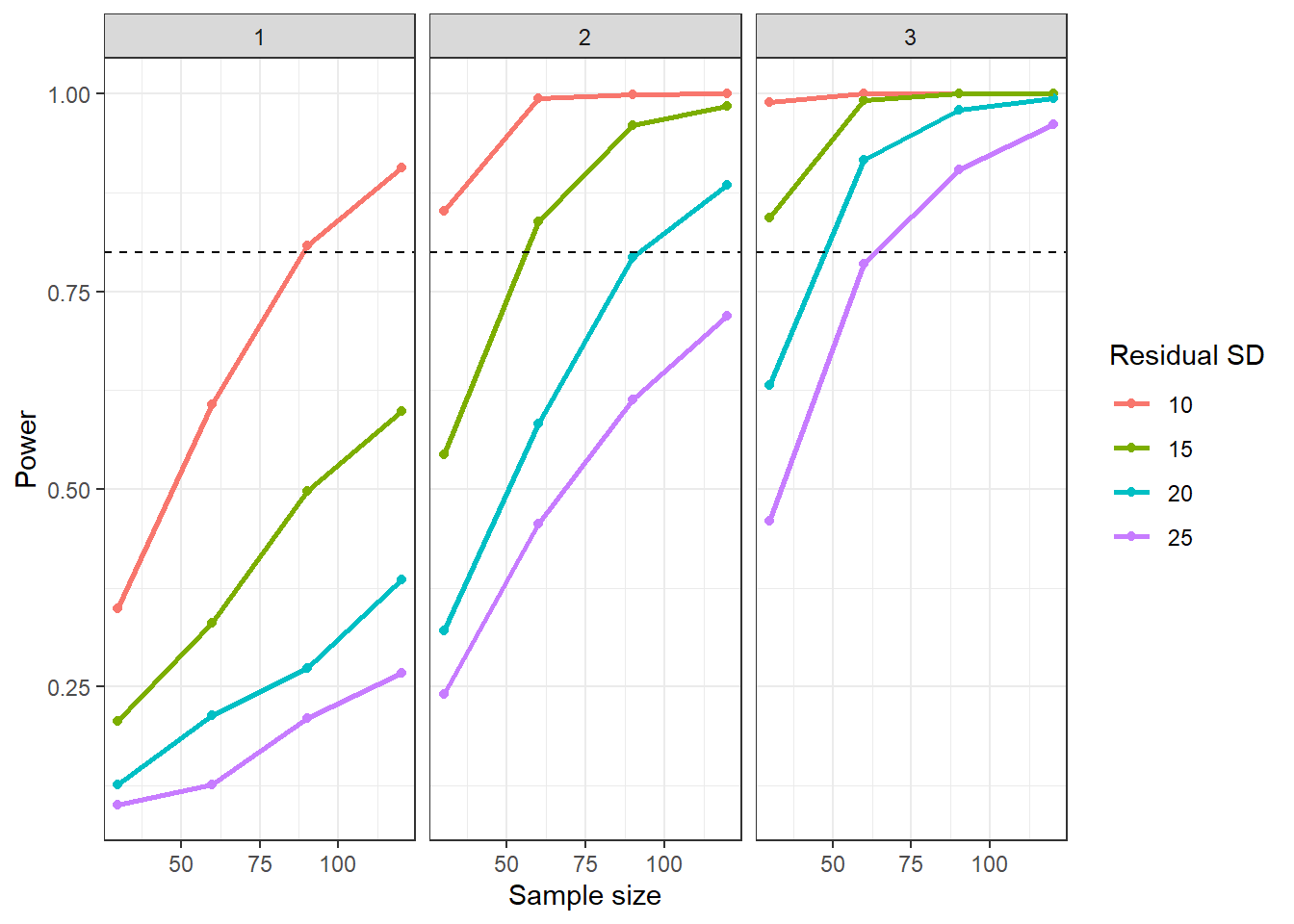
We could also visualise our results in the form of a power contour plot:
ggplot(results, aes(x = n, y = sdi, z = power)) +
  geom_contour_filled() +
  geom_contour(breaks = 0.8, colour = "red", linewidth = 1) +
  facet_wrap(~b1) +
  labs(
    x = "Sample size (n)",
    y = "Residual SD",
    fill = "Power"
  )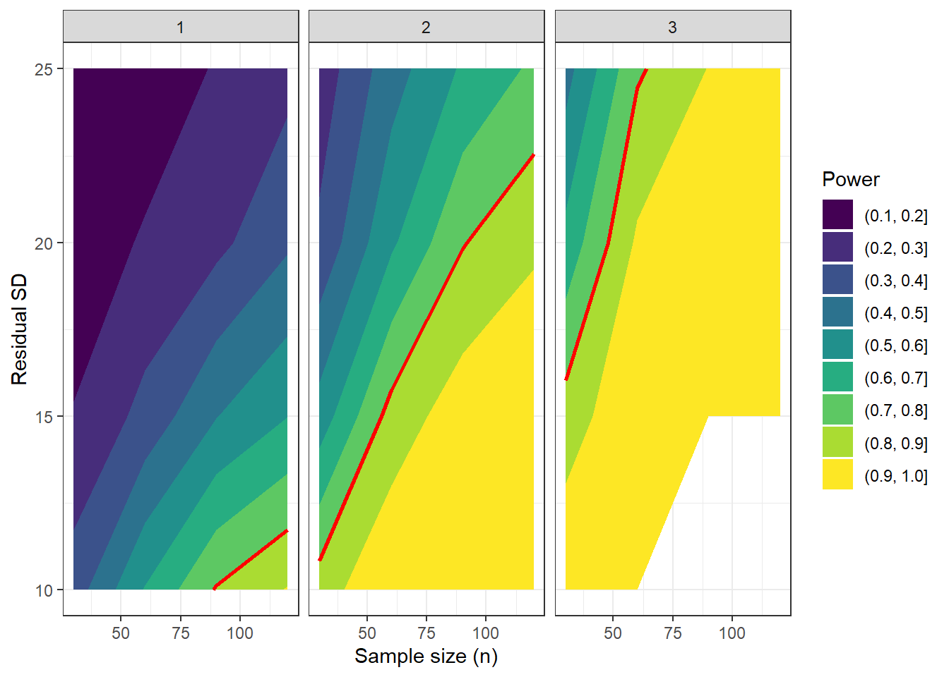
The bands of colour represent contours of power. Anything below and left of the red lines - i.e., the two most yellow contours - signify regions above 80% power.
If we’re feeling really fancy, we can even use the plotly package to produce a 3D plot.
In the code below, we add a new 3D surface for each value of b1 that we’ve tried.
library(plotly)
Attaching package: 'plotly'The following object is masked from 'package:downlit':
highlightThe following object is masked from 'package:MASS':
selectThe following object is masked from 'package:ggplot2':
last_plotThe following object is masked from 'package:stats':
filterThe following object is masked from 'package:graphics':
layoutplot_ly(results,
x = ~n,
y = ~sdi,
z = ~b1,
color = ~power,
type = "scatter3d", mode = "markers") %>%
layout(scene = list(
xaxis = list(title = "Sample size (n)"),
yaxis = list(title = "Residual SD"),
zaxis = list(title = "Effect size (b1)")))When we visualise with these contour plots, 2D or 3D, we give ourselves wiggle room to perhaps test a few more combinations of parameters and still be able to interpret our simulation results meaningfully.
(In fact, our 3D plot would probably benefit from this!)
You could set that up like so, and then rerun the nested loop above - note, this will be notably slower.
nsim <- 1000

n_vals <- seq(20, 200, by = 25)
sdi_vals <- seq(10, 30, by = 5)
b1_vals <- seq(1, 3, by = 0.5)

b0 <- 175

results <- expand.grid(n = n_vals,
                       sdi = sdi_vals,
                       b1 = b1_vals)

results$power <- NA
10.4 More complex models
In the example above, we ran a power analysis by simulation for a model with just one predictor.
Let’s now look at a more complex situation, clutchsize ~ length*pond.
NoteWhich p-values should we track?
Now that we have multiple predictors, we also have multiple p-values we can assess.
As before, we’re probably interested in the overall model versus the null. We’ll need to do a little extra work to find that p-value as you’ll see below.
However, we also have three terms in our model: the two main effects, plus our interaction effects.
We will track the pond and pond:length p-values in our new nested loop.
For this simulation, we won’t bother tracking the main effect of length, our continuous predictor.
The beta coefficient for the length variable only has a clear interpretation if the interaction is zero (which it won’t be), or if we’re evaluating solely at the reference group for pond.
nsim <- 1000

p_overall <- numeric(nsim)
p_pond <- numeric(nsim)
p_inter <- numeric(nsim)

n <- 60
b0 <- 175
b1 <- 2
b2 <- c(0,30,-10)
b3 <- c(0,0.5,-0.2)
sdi <- 20

for(i in 1:nsim){

  length <- rnorm(n, 48, 3)
  pond <- factor(rep(c("A","B","C"), each = n/3))

  avg_clutch <- b0 +
                b1*length +
                model.matrix(~0+pond) %*% b2 +
                model.matrix(~0+length:pond) %*% b3

  clutchsize <- rnorm(n, avg_clutch, sdi)
  dat <- data.frame(clutchsize, length, pond)

  lm_toads <- lm(clutchsize ~ length*pond, data = dat)
  a <- anova(lm_toads)
  s <- summary(lm_toads)

  p_overall[i] <- pf(s$fstatistic[1],
                     s$fstatistic[2],
                     s$fstatistic[3],
                     lower.tail = FALSE)
  p_pond[i] <- a["pond", "Pr(>F)"]
  p_inter[i] <- a["length:pond", "Pr(>F)"]
}

power_overall <- mean(p_overall < 0.05)
power_pond <- mean(p_pond < 0.05)
power_inter <- mean(p_inter < 0.05)

power_overall
[1] 1power_pond[1] 1power_inter[1] 0.051The interaction effect has much, much lower power than the model as a whole, or the main effect of pond.
This means that if we care about this interaction, we should be focusing on its power when designing our experiment. Looking at the model as a whole will not be enough!
10.5 Exercises
10.5.1 Exercise 1 - A priori power analysis
10.6 Summary
TipKey Points
- Turning a dataset simulation into a power analysis just requires a for loop, where the p-value is calculated and saved each time
- This gives more flexibility in the power analysis, allowing you to sweep across different parameter values, and assess power for individual predictors as well as the model as a whole