library(tidyverse)
library(rstatix)5 The central limit theorem
Now that you have the programming basics, we’re going to use them to make sense of a famous statistical concept: the central limit theorem.
5.1 Libraries and functions
NoteClick to expand
import pandas as pd
import numpy as np
import random
import statistics
import matplotlib.pyplot as plt
import statsmodels.stats.api as sms
from scipy.stats import t
5.2 Estimating parameters from datasets
There are two main forms of statistical inference, from dataset to population.
- Estimating parameters
- Testing hypotheses
We’ll get onto the second form later on, but for this section, we’re going to focus on estimating parameters.
In other words - can we do a good job of recreating the distribution of the underlying population, just from the sample we’ve taken from that population?
Our ability to do this well often hinges on the quality of our sample. This includes both the size of the sample, and whether it is biased in any way.
If our sample is biased, there’s not much we can do about it apart from a) scrapping it and starting again, or b) acknowledging the uncertainty/narrowed focus of our conclusions.
We do, however, often have some control over the sample size. Let’s look at how sample size affects our parameter estimates.
5.2.1 Mean
When simulating data, we have an unusual level of knowledge and power (in the normal sense of the word, not the statistical one!):
We know exactly what the true population parameters are, because we specified them.
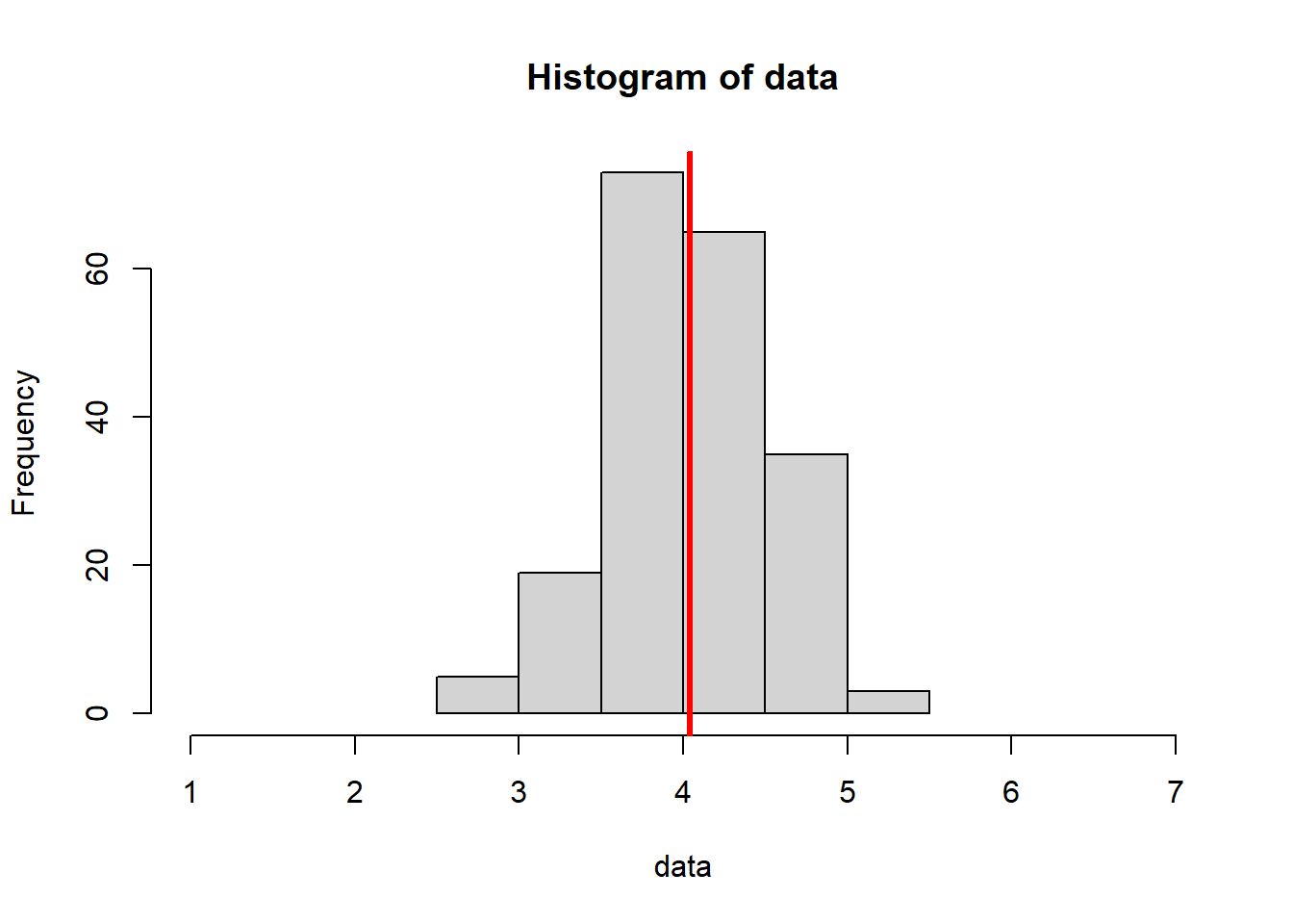
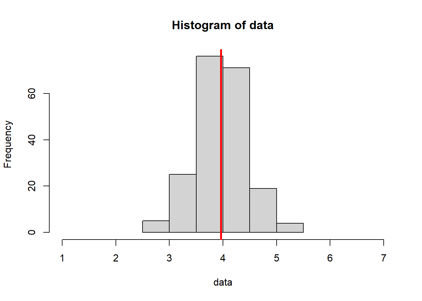
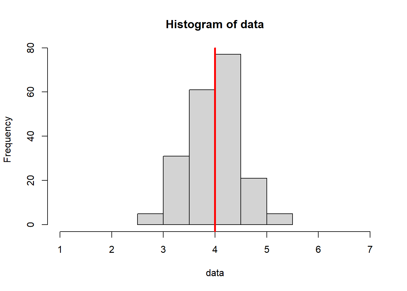
In the code below, we know that the actual true population mean is 4, with no uncertainty. We have set this to be the “ground truth”.
This code is similar to the for loop introduced in Section 4.3.2, but we’ve increased the sample size.
Notice how this:
- Decreases variance (our histograms are “squished” inward - pay attention to the x axis scale)
- Increases the consistency of our mean estimates (they are more similar to one another)
- Increases the accuracy of our mean estimates (they are, overall, closer to the true value of 4)
for (i in 1:3) {

  n <- 200
  mean_n <- 4
  sd_n <- 0.5

  data <- rnorm(n, mean_n, sd_n)

  hist(data, xlim = c(1, 7)); abline(v = mean(data), col = "red", lwd = 3)

  }
for i in range(1, 4):
  n = 200
  mean = 4
  sd = 0.5
  data = np.random.normal(mean, sd, n)
  plt.figure()
  plt.hist(data)
  plt.axvline(x = statistics.mean(data), color = 'r')
  plt.show()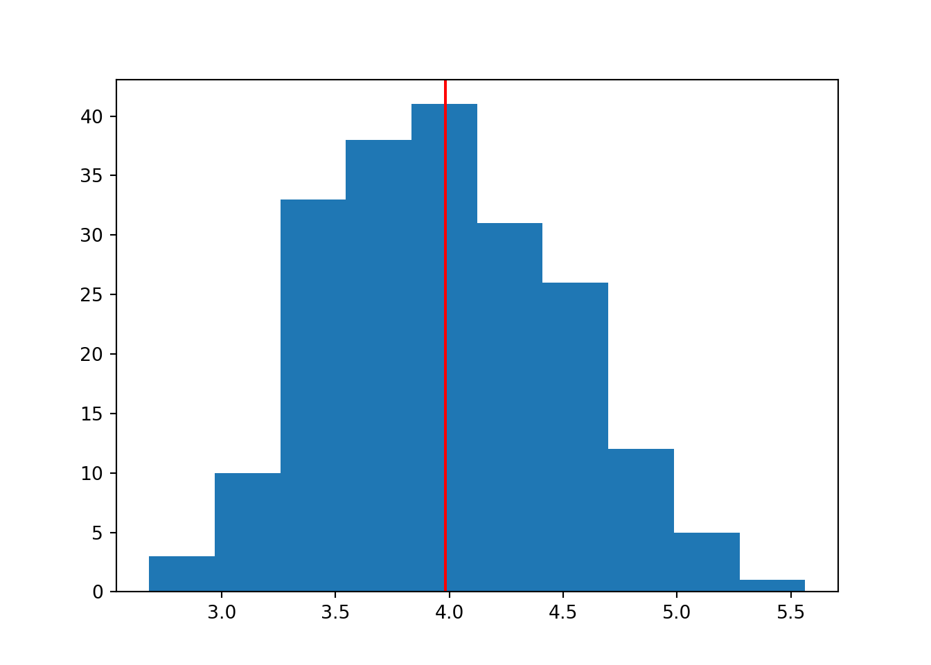
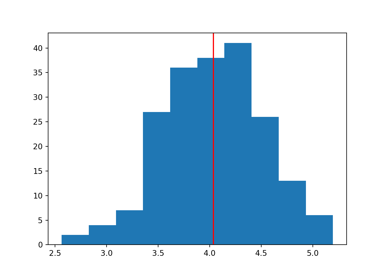
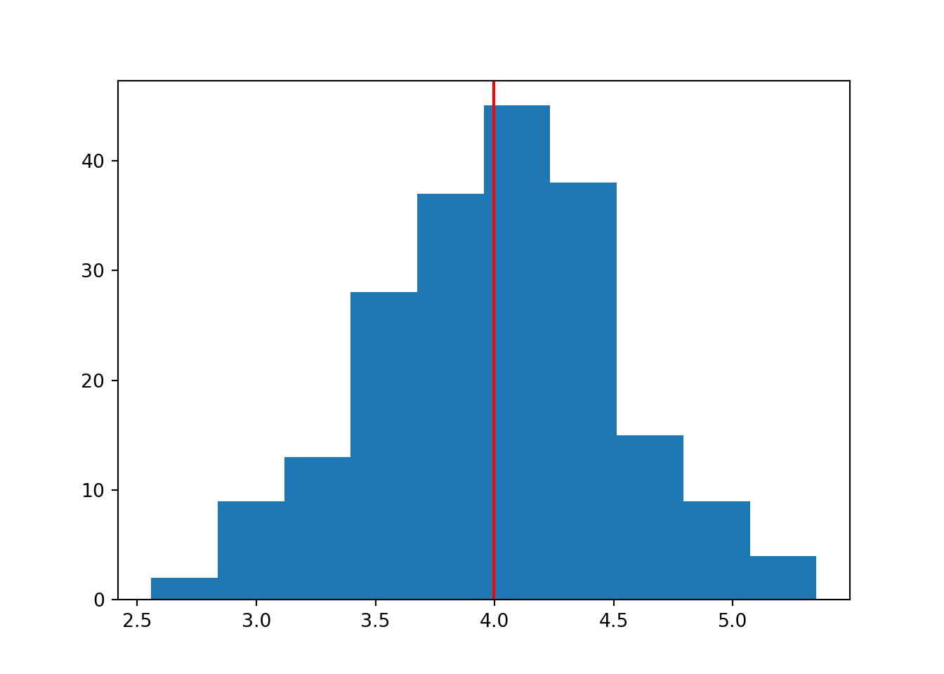
In a larger sample size, we are able to do a better job of “recovering” or recreating the original parameter we specified.
TipThe average of averages
When we take multiple samples and average across them, we do an even better job of recovering the true population mean.
In other words, if we sampled a bunch of datasets, and then took the average of all of their respective means, we’d probably get pretty close to 4.
The section later on in this chapter, on the central limit theorem, pushes this idea a little further.
5.2.2 Variance
In the code above, we also know what the true population variance is, because we set it (by setting standard deviation, the square root of variance).
TipWhat do we mean by “variance”?
Variance is calculated by measuring the difference from each data point and the mean, squaring them, adding those squares up, and then dividing by the number of data points. The mathematical formula looks like this:
\[ \text{Var}(X) = \frac{ \sum_{i=1}^{n} (x_i - \bar{x})^2 } {n} \]
However, when we estimate population variance from a sample, we actually tweak this formula a bit. We divide instead by \(n - 1\):
\[ \text{Var}(X) = \frac{ \sum_{i=1}^{n} (x_i - \bar{x})^2 } {n - 1} \]
Why?
Well, I could give you a theoretical explanation. Or, we can use the power of simulation, and see for ourselves more intuitively.
For the next section, the word variance will crop up in different forms:
- Estimated sample variance, calculated by dividing by \(n - 1\), from a dataset
- Estimated variance, calculated by dividing by \(n\), from a dataset
- The true population variance, which isn’t calculated; it’s known/specified by us
In the for loop below, we are using the same simulation parameters as above, and calculating (manually) two types of variance.
We’ll set the mean to 4 and the variance to 1:
results <- data.frame(var=numeric(),
                      sample_var=numeric())

for (i in 1:30) {

  n <- 10
  mean_n <- 4
  sd_n <- 1

  data <- rnorm(n, mean_n, sd_n)

  v <- sum((data - mean(data))^2)/n
  samplev <- sum((data - mean(data))^2)/(n-1)

  results <- rbind(results, data.frame(var = v, sample_var = samplev))

}
To break down this code further:
We’ve initialised a results table with our desired columns first. On each iteration of the loop (30 total), we sample a dataset, calculate the estimated variance estv and sample variance samplev using slightly different formulae, and then add them to our results table.
rows = []

for i in range(30):
    n = 10
    mean = 4
    sd = 1

    data = np.random.normal(mean, sd, n)

    v = np.sum((data - np.mean(data))**2) / n
    samplev = np.sum((data - np.mean(data))**2) / (n - 1)

    rows.append({'var': v, 'sample_var': samplev})

results = pd.DataFrame(rows)
To break down this code further:
On each iteration of the loop (30 total), we sample a dataset, calculate the estimated variance estv and sample variance samplev using slightly different formulae. These values are collated by our rows object, which we finally convert to a pandas dataframe (a results table).
Now, let’s look at those results and what they show us.
First, we’ll create a new column in our results object that contains the difference between our estimates in each case.
results <- results %>%
mutate(diff_var = sample_var - var)results['diff_var'] = results['sample_var'] - results['var']When we look at the final results file, we see that the estimated sample variance is, on average, a bit bigger than the estimated variance. This makes sense, because we’re dividing by a smaller number when we calculate the sample variance (in other words, \(n - 1 < n\)).
Now, let’s look at the average variance and sample variance, and see which of them is doing the best job of recreating our true population variance (which we know is 1, because we built the simulation that way).
results %>%
  summarise(mean(var), mean(sample_var), mean(diff_var))
mean(var) mean(sample_var) mean(diff_var)
1 0.9183643 1.020405 0.1020405summary = results[['var', 'sample_var', 'diff_var']].mean()
print(summary)var 0.918773
sample_var 1.020859
diff_var 0.102086
dtype: float64Here, we’ve taken the mean of each column. This means we’re looking at the average estimated variance and the average estimated sample variance, across all 10 of our random datasets.
TipRemember, each of these numbers is an average
Yes, now we’re taking the mean of the variance. Yes, we could also measure the variance of the variance if we wanted. Yes, this does start to get confusing the more you think about it.
More on this in the central limit theorem section!
As we can see from these results, when the sample size is small, our estimated variance (on average) underestimates the true value.
This is because, the smaller the sample, the less likely it is to contain values from the edges or tails of the normal distribution, so we don’t get a good picture of the true spread.
The sample variance accounts for this by dividing by n - 1 instead, so the estimate is larger and less of an underestimate.
To get an intuition for this, let’s repeat all the code above, but with a larger sample size:
results <- data.frame(var=numeric(),
sample_var=numeric())
for (i in 1:30) {
n <- 20
mean_n <- 4
sd_n <- 1
data <- rnorm(n, mean_n, sd_n)
v <- sum((data - mean(data))^2)/n
sample <- sum((data - mean(data))^2)/(n-1)
results <- rbind(results, data.frame(var = v, sample_var = sample))
}
results <- results %>%
mutate(diff_var = sample_var - var)
results %>%
summarise(mean(var), mean(sample_var), mean(diff_var)) mean(var) mean(sample_var) mean(diff_var)
1 0.9507581 1.000798 0.0500399rows = []
for i in range(30):
n = 20
mean = 4
sd = 1
data = np.random.normal(mean, sd, n)
v = np.sum((data - np.mean(data))**2) / n
samplev = np.sum((data - np.mean(data))**2) / (n - 1)
rows.append({'var': v, 'sample_var': samplev})
results = pd.DataFrame(rows)
results['diff_var'] = results['sample_var'] - results['var']
summary = results[['var', 'sample_var', 'diff_var']].mean()
print(summary)
var 0.953684
sample_var 1.003878
diff_var 0.050194
dtype: float64When n is larger, notice how the estimated variance is now closer to the true population variance, on average?
With a larger sample size, we are more likely to sample the full “spread” of the distribution.
The estimated sample variance, however, is about as close to the true population variance as it was before, and so the difference between the estimated variance and estimated sample variance has shrunk.
TipWhy sample variance is even cleverer than you might think
Dividing by n - 1 has a bigger impact when the sample is small, where 1 will be a relatively larger fraction of n.
This is great, because these smaller samples are also the place where we need this adjustment most: they’re less likely to contain values from the tails of the distribution, and therefore will underestimate the true population variance more.
In contrast, when our sample is much bigger, it’s going to be more representative/less noisy, and we see much less of an underestimation and will need less adjustment. Happily, we will automatically get less of an adjustment anyway, since the 1 is now a smaller fraction of n.
In other words: the impact of dividing by n - 1 scales naturally with both the size of n, and with the amount of underestimation we need to account for.
In fact, when the sample is infinitely large, we should see no difference between the estimated sample variance and the estimated variance at all, because n-1 = n at infinity.
You can test this intuition (except for the infinity part, you kinda just have to trust me on that) by continuing to mess around with the value of n in the code above.
Since sample variance is the most effective way to estimate the true population variance, functions in R and Python will default to this.
The var function in R specifically calculates the sample variance. We can see that we get identical results using the function or doing it manually, by adapting the loop above:
results <- data.frame(var=numeric(),
                      sample_var=numeric(),
                      r_var=numeric())

for (i in 1:30) {

  n <- 20
  mean_n <- 4
  sd_n <- 1

  data <- rnorm(n, mean_n, sd_n)

  v <- sum((data - mean(data))^2)/n
  sample <- sum((data - mean(data))^2)/(n-1)

  # Add an extra column containing the results of var(data)
  results <- rbind(results, data.frame(var = v, sample_var = sample, r_var = var(data)))

}

results %>%
  summarise(mean(var), mean(sample_var), mean(r_var))
mean(var) mean(sample_var) mean(r_var)
1 0.9507581 1.000798 1.000798Notice how mean(sample_var) and mean(r_var) are identical?
The numpy.var function specifically calculates sample variance. We can see that we get identical results using the function or doing it manually, by adapting the loop above:
rows = []

for i in range(30):
    n = 20
    mean = 4
    sd = 1

    data = np.random.normal(mean, sd, n)

    # Estimated variance
    v = np.sum((data - np.mean(data))**2) / n
    # Sample variance
    sample = np.sum((data - np.mean(data))**2) / (n - 1)
    # numpy sample variance
    np_var = np.var(data, ddof=1)

    rows.append({'var': v, 'sample_var': sample, 'np_var': np_var})

results = pd.DataFrame(rows)

summary = results[['var', 'sample_var', 'np_var']].mean()
print(summary)
var 0.953684
sample_var 1.003878
np_var 1.003878
dtype: float64Notice how sample_var and np_var are identical?
5.3 Central limit theorem
In the section above, we used for loops to simulate multiple datasets, measure certain statistics from them, and then averaged those statistics across the datasets.
So, in some cases, we were looking at the mean of the means, or the mean of the variances. We’re going to unpack that a bit further now.
Specifically, we’re going to talk about the central limit theorem: the idea that, across multiple samples taken from the same distribution, the estimates/statistics we calculate from them will themselves follow a normal distribution.
5.3.1 An example: the mean
You will recognise all the code below from previous sections, but here we’re using it to show us a slightly different distribution.
Instead of producing separate histograms for each of the datasets (i.e., one per loop), we are instead simply collecting the mean value from each of our datasets.
Then, we will treat the set of means as a sample in itself, and visualise its distribution.
means <- c()

for (i in 1:40) {

  n <- 200
  mean_n <- 4
  sd_n <- 1

  means[i] <- mean(rnorm(n, mean_n, sd_n))

}

hist(means)
abline(v = mean(means), col = "red", lwd = 3)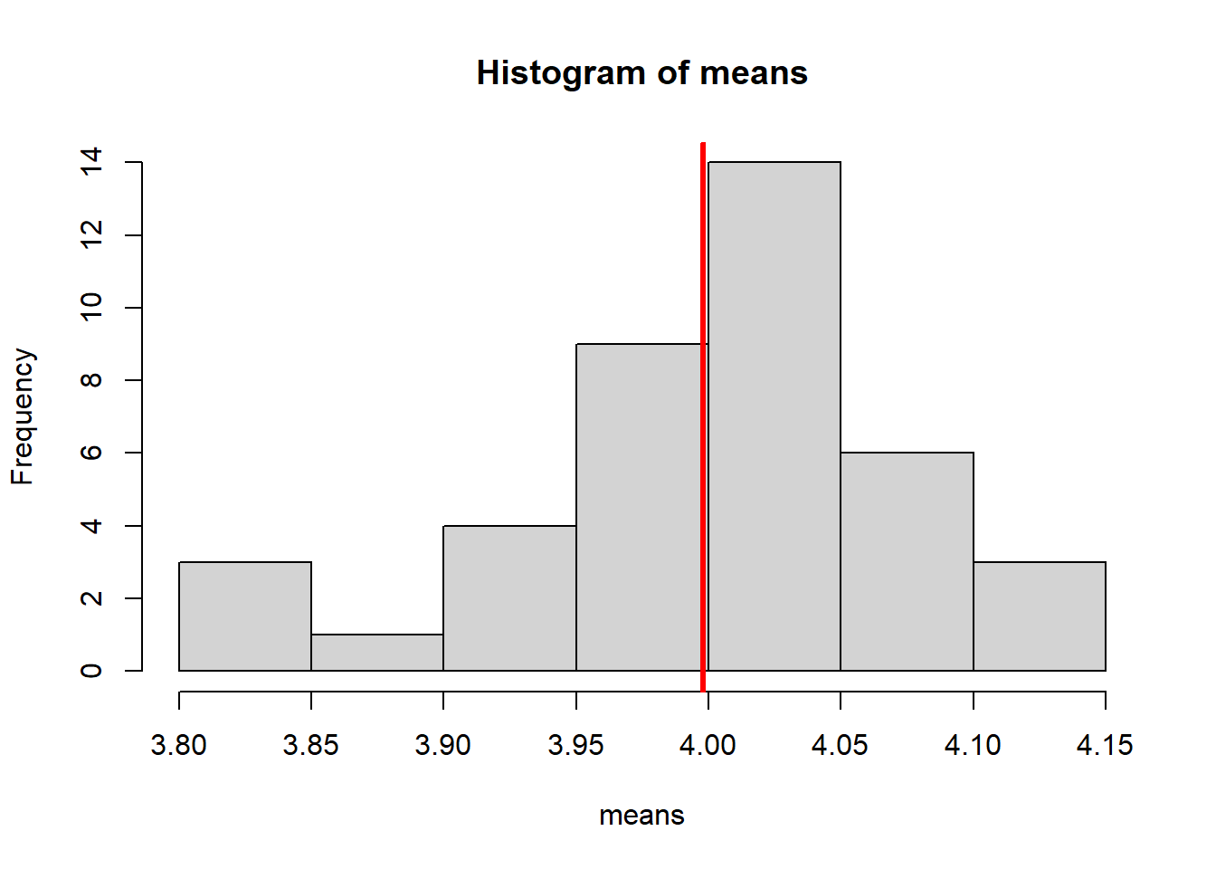
means = []

for i in range(40):
  n = 200
  mean = 4
  sd = 1

  est_mean = np.random.normal(mean, sd, n).mean()

  means.append(est_mean)

plt.clf()
plt.hist(means)
plt.axvline(x = statistics.mean(means), color = 'r')
plt.show()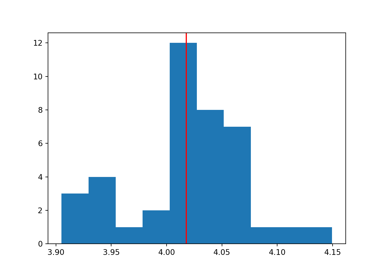
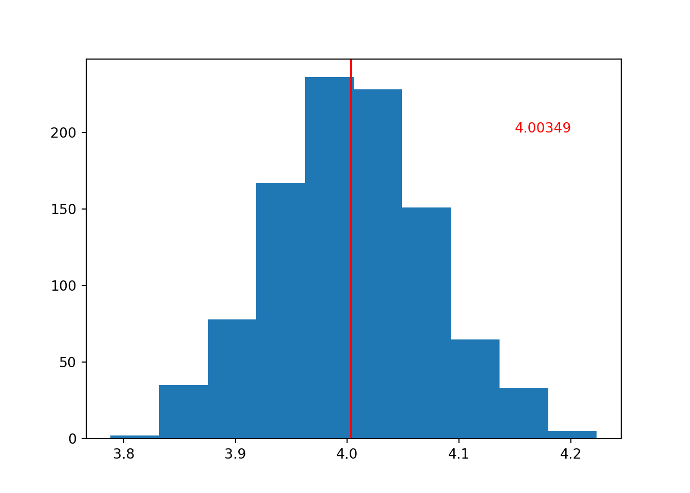
The set of means from our i datasets, follow a normal distribution. The mean of this normal distribution is approximately the true population mean (which we know to be 4).
If we increase the number of iterations/loops, we will sample more datasets, with more means.
If we think of our set of sample means as a sample in itself, then doing this is effectively increasing our sample size. And, as we know from the first section of this chapter, that means that the mean of our distribution should be a better estimate of the true population value.
This is exactly what happens:
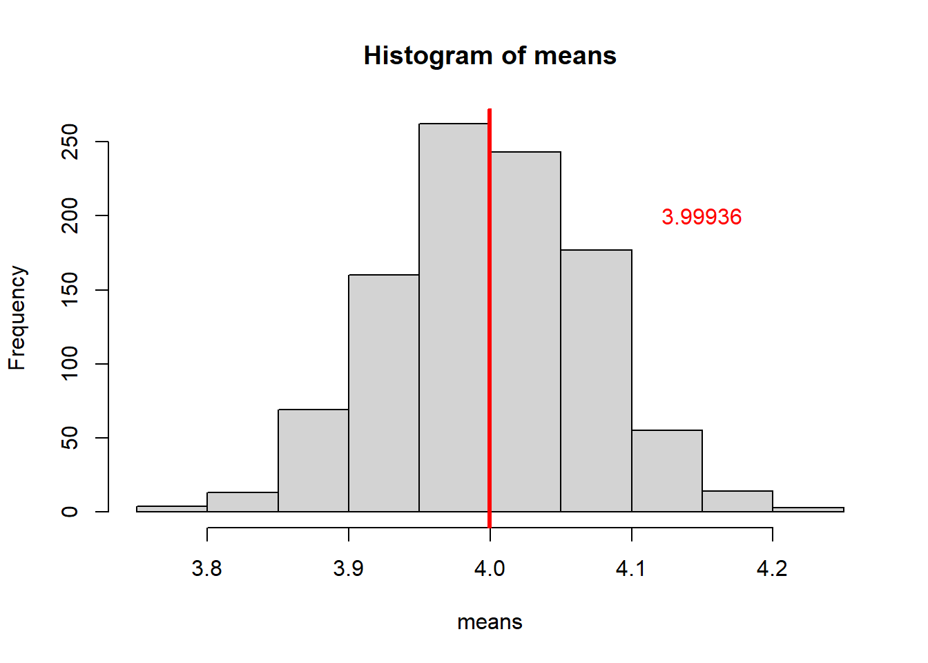
To produce the plot above, the number of iterations was set to i = 1000.
Try setting it to something between 40 and 1000, or even more than 1000, and see how that changes things.
TipStandard error of the mean
You may have come across the concept of the standard error of the mean in the past (especially when constructing error bars for plots). But now, you should be in a better position to really understand what it is.
In the histogram above, we’ve calculated the mean of the sample means. But around that mean of sample means, there is some spread or noise.
We can quantify that spread by measuring the standard deviation of the distribution of sample means - and if we do, we’ve calculated the standard error.
Of course, in classical statistics we usually only have one dataset, rather than 1000, to help us figure out that standard error. So, like with everything else we calculate from a dataset, we are only ever able to access an estimate of that standard error.
5.3.2 It’s always normal
The really quirky thing about the central limit theorem is that it doesn’t actually matter what distribution you pulled the original samples from. In other words, the results we got above aren’t just because we were using the normal distribution for our simulations.
To prove that, the code here has been adapted to pull each of our 1000 samples from a uniform distribution instead, and estimate the mean.
Note the use of runif instead of rnorm:
means <- c()

for (i in 1:1000) {

  n <- 200
  min_n <- 1
  max_n <- 7

  means[i] <- mean(runif(n, min_n, max_n))

}

hist(means)
abline(v = mean(means), col = "red", lwd = 3)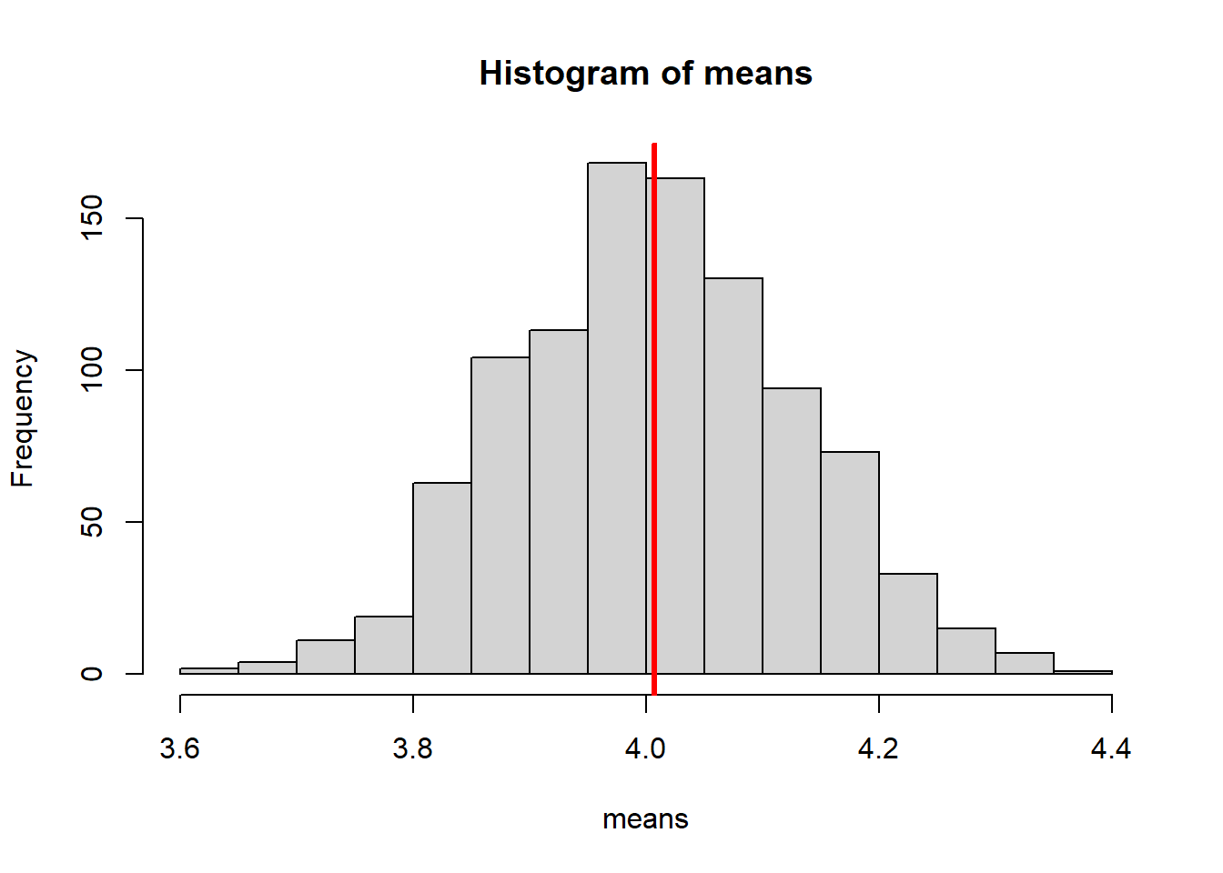
Note the use of np.random.uniform instead of np.random.normal:
means = []

for i in range(1000):
  n = 200
  lower = 1
  upper = 7
  est_mean = np.random.uniform(mean, sd, n).mean()
  means.append(est_mean)

plt.clf()
plt.hist(means)
plt.axvline(x = statistics.mean(means), color = 'r')
plt.show()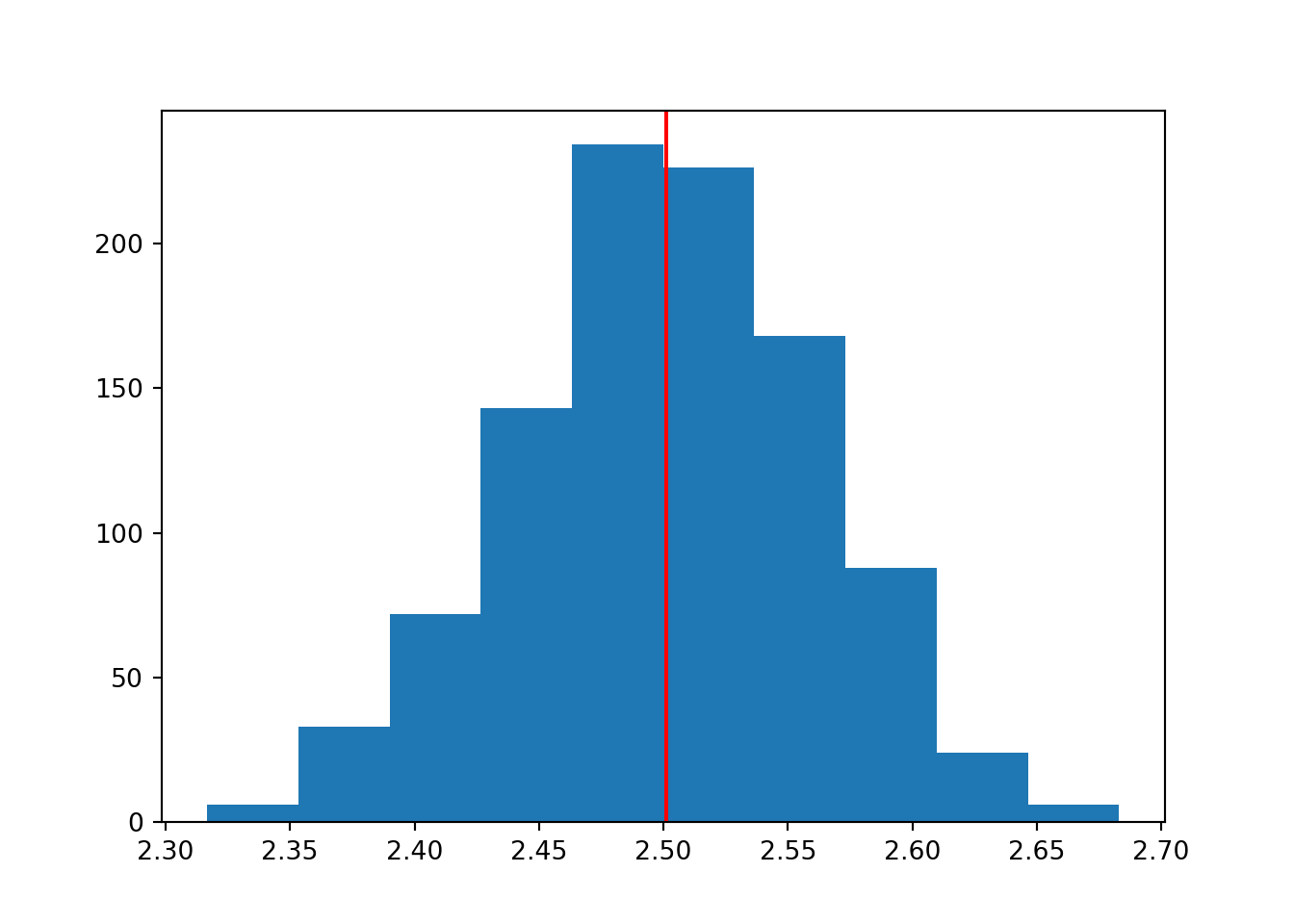
Although each of the individual samples would have a flat histogram, that’s not what we’re plotting here. Here, we’re looking at the set of means that summarise each of those individual samples.
The nature of the underlying population distribution doesn’t matter - the distribution of the parameter estimates is still normal, which we can see clearly with a sufficient number of simulations.
No wonder the normal distribution enjoys such special status in statistics.
5.4 Exercises
5.4.1 t-statistic under CLT
All statistics obey the central limit theorem. This includes not just descriptive statistics like the mean, median, standard deviation etc., but the test statistics that we use for hypothesis testing.
5.4.2 Distributions all the way down
Those of you with imagination might be wondering: if one for loop can construct a single histogram, giving us the distribution of the set of sample means, why can’t we run multiple for loops and look at the distribution of the set of means of the set of means?
The short answer is: we can!

ExerciseExercise 2
Level:
Your mission, should you choose to accept it, is to plot a single histogram that captures the distribution of the set of means of the set of means.
Adapt the code in Section 5.3.1 by nesting one for loop inside the other, to produce a single histogram. It should represent the set of means of the set of sample means.
Before you do, consider:
- What shape will the histogram take, if you run enough iterations?
- If someone asks what you did on this course, how on earth will you explain this to them?!
TipWorked answer
To make the code a little easier to parse and eliminate any clashes in the environment, the outside for loop uses j for indexing instead of i.
We’ve also kept the number of iterations low-ish. You might notice, if you use a large value like 1000 for each of the loops, it takes a while to run (because you’re actually asking for 1000000 total iterations!)
means_j <- c()

for (j in 1:300) {

  means_i <- c()

  for (i in 1:300) {

    n <- 20
    min_n <- 1
    max_n <- 7

    means_i[i] <- mean(runif(n, min_n, max_n))

  }

  means_j[j] <- mean(means_i)

}

hist(means_j)
abline(v = mean(means_j), col = "red", lwd = 3)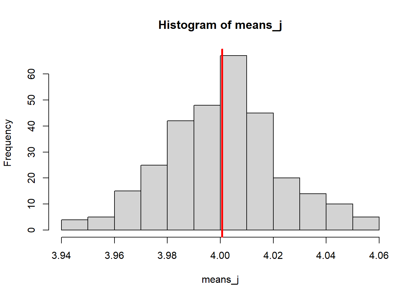
means_j = []

for j in range(300):

  means_i = []

  for i in range(300):
    n = 20
    lower = 1
    upper = 7
    imean = np.random.uniform(lower, upper, n).mean()
    means_i.append(imean)

  jmean = np.mean(means_i)
  means_j.append(jmean)

plt.clf()
plt.hist(means_j)
plt.axvline(x = np.mean(means_j), color = 'r')
plt.show()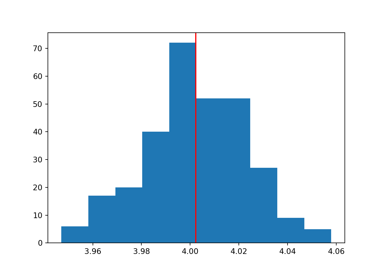
It’s still normal. If this is what you guessed, well done.
If you were to take this further, and add an infinite number of nested loops, you’d get a normal distribution each time.
And it doesn’t even matter what distribution we sample our individual datasets from, as we showed above. In this worked example code we’ve used the uniform distribution, but you can try swapping it out for any other distribution - you’ll still get a normal distribution at each “layer”, which gets clearer and clear the more iterations you run.
Now, statistics may not be considered the “coolest” subject in the world - but I think that’s pretty awesome, don’t you?
5.5 Summary
Simulation is a great way to help get your head around more difficult or abstract statistical concepts, without needing to worry about the mathematical formulae.
The central limit theorem is incredibly boring to explain via equations, and much less easy to get your head around - so why not just simulate?
TipKey Points
- We are more likely to accurately and precisely “recover” the true population parameters when our sample is large and unbiased
- The central limit theorem shows that, across a number of samples, the set of estimates of a given parameter will follow an approximately normal distribution
- When the number of samples = \(\infty\), it will be perfectly normal
- This is true regardless of the original distribution that the individual samples come from