library(tidyverse)
library(rstatix)

library(performance)
library(ggResidpanel)9 Simulating interactions
9.1 Libraries and functions
NoteClick to expand
import numpy as np
import pandas as pd
import matplotlib.pyplot as plt
import seaborn as sns

import statsmodels.api as sm
import statsmodels.formula.api as smf
import pingouin as pg

from patsy import dmatrix
In this chapter, we’re going to simulate a few different possible interactions for the goldentoad dataset we’ve been building.
As with main effects, categorical interactions are a little trickier than continuous ones, so we’ll work our way up.
9.2 Two continuous predictors
The easiest type of interaction to simulate is a two-way interaction between continuous predictors.
We’ll use the length predictor from before, and add a new continuous predictor, temperature.
(I don’t know whether temperature actually does predict clutch size in toads - remember, this is made up!)
Set up parameters and predictors
First, we set the important parameters. This includes the beta coefficients.
NoteYou might notice…
… that we’ve increased the sample size from previous chapters, and tweaked beta0.
This is to give our model a fighting chance to recover some sensible estimates at the end, and also to keep the values of our final clutchsize variable within some sensible biological window.
However, all of this is optional - the process of actually doing the simulation would work the same even with the old values!
set.seed(22)

n <- 120
b0 <- -30             # intercept
b1 <- 0.7               # main effect of length
b2 <- 0.5             # main effect of temperature

b3 <- 0.25             # interaction of length:temperature

sdi <- 12np.random.seed(28)
n = 120
b0 = -30 # intercept
b1 = 0.7 # main effect of length
b2 = 0.5 # main effect of temperature
b3 = 0.25 # interaction of length:temperature
sdi = 12Notice that the beta coefficient for the interaction is just a single constant - this is always true for an interaction between continuous predictors.
Next, we generate the values for length and temperature:
length <- rnorm(n, 48, 3)

temperature <- runif(n, 10, 32)
length = np.random.normal(48, 3, n)
temperature = np.random.uniform(10, 32, n)Just for a bit of variety, we’ve sampled temperature from a uniform distribution instead of a normal one.
It won’t make any difference at all to the rest of the workflow, but if you’d like, you can test both ways to see whether it has an impact on the visualisation and model at the end!
Simulate response variable
These steps should look familiar from previous chapters.
avg_clutch <- b0 + b1*length + b2*temperature + b3*length*temperature

clutchsize <- rnorm(n, avg_clutch, sdi)

goldentoad <- tibble(length, temperature, clutchsize)
avg_clutch = b0 + b1*length + b2*temperature + b3*length*temperature
clutchsize = np.random.normal(avg_clutch, sdi, n)
goldentoad = pd.DataFrame({'length': length, 'temperature': temperature, 'clutchsize': clutchsize})Check the dataset
First, let’s visualise the dataset.
This isn’t always easy, with two continuous variables, but one way that gives us at least some idea is to assign one of our continuous predictors to the colour aesthetic:
ggplot(goldentoad, aes(x = length, y = clutchsize, colour = temperature)) +
  geom_point(size = 3) +
  scale_colour_continuous(type = "viridis")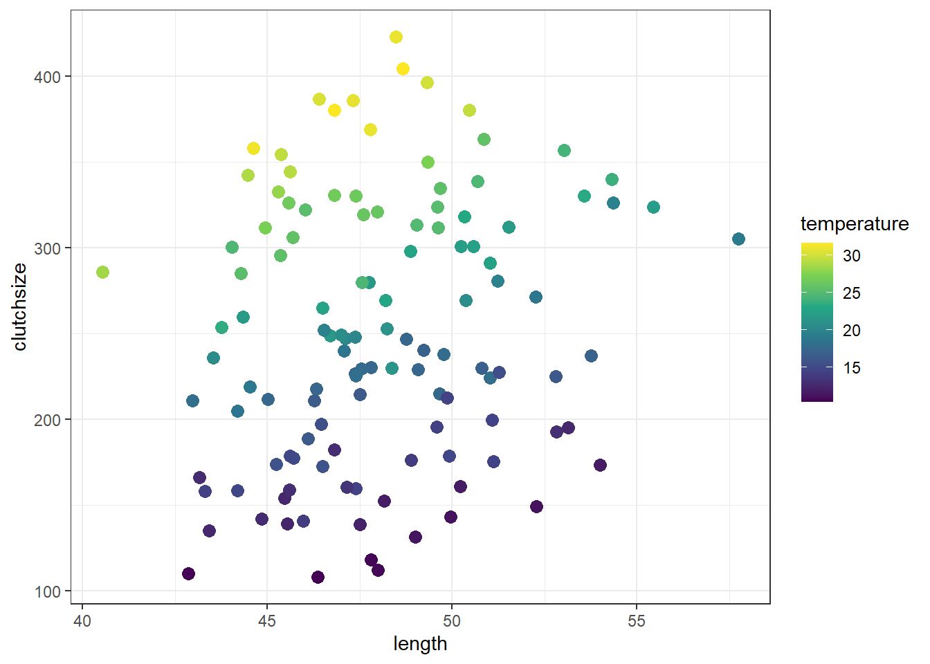
plt.clf()
plt.scatter(goldentoad["length"], goldentoad["clutchsize"], c=goldentoad["temperature"],
    cmap="viridis", s=40)          # optional - set colourmap and point size
# add labels
plt.xlabel("Length"); plt.ylabel("Clutch Size"); plt.colorbar(label="Temperature")
Text(0.5, 0, 'Length')
Text(0, 0.5, 'Clutch Size')
<matplotlib.colorbar.Colorbar object at 0x000001F506C740B0>plt.grid(True)
plt.show()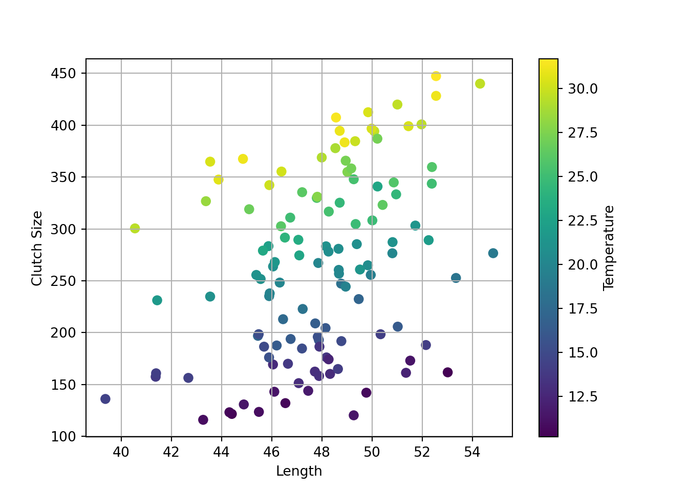
Broadly speaking, clutchsize is increasing with both length and temperature, which is good - we specified positive betas for both main effects.
Since we specified a positive beta for the interaction, we would expect there to be a bigger increase in clutchsize per unit increase in length, for each unit increase in temperature.
Visually, that should look like the beginnings of a “trumpet” or “megaphone” shape in the data; you’re more likely to see that with a larger sample size.
Next, let’s fit the linear model and see if we can recover those beta coefficients:
lm_golden <- lm(clutchsize ~ length * temperature, data = goldentoad)
summary(lm_golden)
Call:
lm(formula = clutchsize ~ length * temperature, data = goldentoad)
Residuals:
Min 1Q Median 3Q Max
-42.480 -8.079 0.191 8.796 36.987
Coefficients:
Estimate Std. Error t value Pr(>|t|)
(Intercept) -60.41655 71.12790 -0.849 0.397404
length 1.23202 1.49139 0.826 0.410448
temperature 0.11301 3.52109 0.032 0.974452
length:temperature 0.26105 0.07404 3.526 0.000606 ***
---
Signif. codes: 0 '***' 0.001 '**' 0.01 '*' 0.05 '.' 0.1 ' ' 1
Residual standard error: 13.05 on 116 degrees of freedom
Multiple R-squared: 0.9718, Adjusted R-squared: 0.9711
F-statistic: 1332 on 3 and 116 DF, p-value: < 2.2e-16model = smf.ols(formula= "clutchsize ~ length * temperature", data = goldentoad)
lm_golden = model.fit()
print(lm_golden.summary()) OLS Regression Results
==============================================================================
Dep. Variable: clutchsize R-squared: 0.984
Model: OLS Adj. R-squared: 0.984
Method: Least Squares F-statistic: 2370.
Date: Mon, 16 Mar 2026 Prob (F-statistic): 7.23e-104
Time: 17:26:51 Log-Likelihood: -458.42
No. Observations: 120 AIC: 924.8
Df Residuals: 116 BIC: 936.0
Df Model: 3
Covariance Type: nonrobust
======================================================================================
coef std err t P>|t| [0.025 0.975]
--------------------------------------------------------------------------------------
Intercept -16.2454 54.243 -0.299 0.765 -123.681 91.190
length 0.3842 1.138 0.338 0.736 -1.870 2.639
temperature -0.6613 2.488 -0.266 0.791 -5.589 4.267
length:temperature 0.2755 0.052 5.313 0.000 0.173 0.378
==============================================================================
Omnibus: 1.282 Durbin-Watson: 2.077
Prob(Omnibus): 0.527 Jarque-Bera (JB): 0.818
Skew: 0.072 Prob(JB): 0.664
Kurtosis: 3.378 Cond. No. 5.58e+04
==============================================================================
Notes:
[1] Standard Errors assume that the covariance matrix of the errors is correctly specified.
[2] The condition number is large, 5.58e+04. This might indicate that there are
strong multicollinearity or other numerical problems.Not bad. Not brilliant, but not terrible!
Out of interest, let’s also fit a model that we know is incorrect - one that doesn’t include the interaction effect:
lm_golden <- lm(clutchsize ~ length + temperature, data = goldentoad)
summary(lm_golden)
Call:
lm(formula = clutchsize ~ length + temperature, data = goldentoad)
Residuals:
Min 1Q Median 3Q Max
-41.767 -9.325 0.651 9.986 37.804
Coefficients:
Estimate Std. Error t value Pr(>|t|)
(Intercept) -301.4146 20.5996 -14.63 <2e-16 ***
length 6.3030 0.4131 15.26 <2e-16 ***
temperature 12.5066 0.2113 59.18 <2e-16 ***
---
Signif. codes: 0 '***' 0.001 '**' 0.01 '*' 0.05 '.' 0.1 ' ' 1
Residual standard error: 13.68 on 117 degrees of freedom
Multiple R-squared: 0.9688, Adjusted R-squared: 0.9682
F-statistic: 1815 on 2 and 117 DF, p-value: < 2.2e-16model = smf.ols(formula= "clutchsize ~ length + temperature", data = goldentoad)
lm_golden = model.fit()
print(lm_golden.summary()) OLS Regression Results
==============================================================================
Dep. Variable: clutchsize R-squared: 0.980
Model: OLS Adj. R-squared: 0.980
Method: Least Squares F-statistic: 2872.
Date: Mon, 16 Mar 2026 Prob (F-statistic): 3.65e-100
Time: 17:26:51 Log-Likelihood: -471.49
No. Observations: 120 AIC: 949.0
Df Residuals: 117 BIC: 957.3
Df Model: 2
Covariance Type: nonrobust
===============================================================================
coef std err t P>|t| [0.025 0.975]
-------------------------------------------------------------------------------
Intercept -289.7312 19.003 -15.247 0.000 -327.365 -252.097
length 6.1167 0.403 15.169 0.000 5.318 6.915
temperature 12.5306 0.179 69.955 0.000 12.176 12.885
==============================================================================
Omnibus: 0.723 Durbin-Watson: 2.145
Prob(Omnibus): 0.697 Jarque-Bera (JB): 0.326
Skew: -0.007 Prob(JB): 0.850
Kurtosis: 3.255 Cond. No. 876.
==============================================================================
Notes:
[1] Standard Errors assume that the covariance matrix of the errors is correctly specified.Without the interaction term, our estimates are wildly wrong - or least, much more wrong than they were with the interaction.
This is a really nice illustration of how important it is to check for interactions when modelling data.
9.3 One categorical & one continuous predictor
The next type of interaction we’ll look at is between one categorical and one continuous predictor. This is the type of interaction you’d see in a grouped linear regression.
We’ll use our two predictors from the previous chapters, length and pond.
Set up parameters and predictors
Since at least one of the variables in our interaction is a categorical predictor, the beta coefficient for the interaction will need to be a vector.
Think of it this way: our model with an interaction term will consist of three lines of best fit, each with a different intercept and gradient. The difference in intercepts is captured by b2, and then the difference in gradients is captured by b3.
rm(list=ls()) # optional clean-up
set.seed(20)
n <- 60
b0 <- 175 # intercept
b1 <- 2 # main effect of length
b2 <- c(0, 30, -10) # main effect of pond
b3 <- c(0, 0.5, -0.2) # interaction of length:pond
sdi <- 12
length <- rnorm(n, 48, 3)
pond <- rep(c("A", "B", "C"), each = n/3)del(length, pond, goldentoad, clutchsize, avg_clutch) # optional clean-upnp.random.seed(23)
n = 60
b0 = 175 # intercept
b1 = 2 # main effect of length
b2 = np.array([0, 30, -10]) # main effect of pond
b3 = np.array([0, 0.5, -0.2]) # interaction of length:pond
sdi = 12
length = np.random.normal(48, 3, n)
pond = np.repeat(["A","B","C"], repeats = n//3)Simulating the values for length and pond themselves is no different to how we did it in previous chapters.
Simulate response variable
Once again, we use our two-step procedure to simulate our response variable.
Since our interaction is categorical (i.e., contains a categorical predictor), we will need to create a design matrix for it.
model.matrix(~0+length:pond) length:pondA length:pondB length:pondC
1 51.48806 0.00000 0.00000
2 46.24223 0.00000 0.00000
3 53.35640 0.00000 0.00000
4 44.00222 0.00000 0.00000
5 46.66030 0.00000 0.00000
6 49.70882 0.00000 0.00000
7 39.33085 0.00000 0.00000
8 45.39294 0.00000 0.00000
9 46.61489 0.00000 0.00000
10 46.33338 0.00000 0.00000
11 47.93959 0.00000 0.00000
12 47.54885 0.00000 0.00000
13 46.11562 0.00000 0.00000
14 51.96966 0.00000 0.00000
15 43.43595 0.00000 0.00000
16 46.68772 0.00000 0.00000
17 50.91173 0.00000 0.00000
18 48.08467 0.00000 0.00000
19 47.74265 0.00000 0.00000
20 49.16764 0.00000 0.00000
21 0.00000 48.71006 0.00000
22 0.00000 47.56668 0.00000
23 0.00000 50.16669 0.00000
24 0.00000 49.10972 0.00000
25 0.00000 47.27380 0.00000
26 0.00000 43.58381 0.00000
27 0.00000 46.21152 0.00000
28 0.00000 44.55990 0.00000
29 0.00000 40.57609 0.00000
30 0.00000 46.15947 0.00000
31 0.00000 47.35107 0.00000
32 0.00000 52.77044 0.00000
33 0.00000 52.66843 0.00000
34 0.00000 51.32535 0.00000
35 0.00000 44.70797 0.00000
36 0.00000 42.41818 0.00000
37 0.00000 45.25926 0.00000
38 0.00000 51.73671 0.00000
39 0.00000 48.26356 0.00000
40 0.00000 49.27045 0.00000
41 0.00000 0.00000 45.54455
42 0.00000 0.00000 43.37230
43 0.00000 0.00000 49.66765
44 0.00000 0.00000 46.89291
45 0.00000 0.00000 44.85799
46 0.00000 0.00000 48.05454
47 0.00000 0.00000 50.64563
48 0.00000 0.00000 50.64558
49 0.00000 0.00000 51.07873
50 0.00000 0.00000 46.85607
51 0.00000 0.00000 51.29831
52 0.00000 0.00000 47.90725
53 0.00000 0.00000 48.57102
54 0.00000 0.00000 52.00562
55 0.00000 0.00000 50.19166
56 0.00000 0.00000 48.16861
57 0.00000 0.00000 51.98792
58 0.00000 0.00000 46.77564
59 0.00000 0.00000 45.54523
60 0.00000 0.00000 49.07684
attr(,"assign")
[1] 1 1 1
attr(,"contrasts")
attr(,"contrasts")$pond
[1] "contr.treatment"Xpond_length = dmatrix('0 + C(pond):length', data = {'pond': pond, 'length': length})You’ll notice that this design matrix doesn’t contain 0s and 1s, like the design matrix for pond alone does.
Instead, wherever there would be a 1, it has been replaced with the value of length for that row.
This means that when we multiply our design matrix by our b3, the following happens:
model.matrix(~0+length:pond) %*% b3 [,1]
1 0.000000
2 0.000000
3 0.000000
4 0.000000
5 0.000000
6 0.000000
7 0.000000
8 0.000000
9 0.000000
10 0.000000
11 0.000000
12 0.000000
13 0.000000
14 0.000000
15 0.000000
16 0.000000
17 0.000000
18 0.000000
19 0.000000
20 0.000000
21 24.355031
22 23.783340
23 25.083345
24 24.554860
25 23.636901
26 21.791905
27 23.105761
28 22.279950
29 20.288045
30 23.079737
31 23.675533
32 26.385219
33 26.334215
34 25.662676
35 22.353987
36 21.209091
37 22.629632
38 25.868353
39 24.131782
40 24.635223
41 -9.108910
42 -8.674459
43 -9.933529
44 -9.378583
45 -8.971597
46 -9.610908
47 -10.129127
48 -10.129117
49 -10.215746
50 -9.371214
51 -10.259661
52 -9.581450
53 -9.714204
54 -10.401124
55 -10.038331
56 -9.633721
57 -10.397583
58 -9.355128
59 -9.109046
60 -9.815367np.dot(Xpond_length, b3)array([ 0. , 0. , 0. , 0. ,
0. , 0. , 0. , 0. ,
0. , 0. , 0. , 0. ,
0. , 0. , 0. , 0. ,
0. , 0. , 0. , 0. ,
23.69723922, 25.56805692, 24.80724295, 25.218178 ,
24.36165945, 22.5712357 , 23.79559987, 25.90087231,
24.26045047, 22.16511784, 26.12297997, 24.68656647,
25.09331376, 26.9526521 , 23.17831799, 22.98087259,
20.24065452, 24.22044074, 24.90929324, 23.96619166,
-9.60805335, -10.16156694, -9.8523736 , -9.84697178,
-9.55720565, -9.57273745, -10.22453158, -9.54357916,
-9.34749363, -9.26880686, -9.52734147, -9.71408482,
-9.90728244, -9.67892308, -9.40102973, -8.62056823,
-9.97146844, -9.00445573, -9.50319217, -10.3154426 ])We get no adjustments made for any of the measurements from pond A. This is what we wanted, because this pond is our reference group. The gradient between ‘clutchsize ~ length’ in pond A is therefore kept equal to our b2 value.
We do, however, get adjustments for ponds B and C. These generate a different gradient between clutchsize ~ length for our two non-reference ponds.
We then add this in to our model equation, like so:
avg_clutch <- b0 + b1*length + model.matrix(~0+pond) %*% b2 + model.matrix(~0+length:pond) %*% b3
clutchsize <- rnorm(n, avg_clutch, sdi)
goldentoad <- tibble(clutchsize, length, pond)Xpond = dmatrix('0 + C(pond)', data = {'pond': pond})
Xpond_length = dmatrix('0 + C(pond):length', data = {'pond': pond, 'length': length})
avg_clutch = b0 + b1*length + np.dot(Xpond, b2) + np.dot(Xpond_length, b3)
clutchsize = np.random.normal(avg_clutch, sdi, n)
goldentoad = pd.DataFrame({'pond': pond, 'length': length, 'clutchsize': clutchsize})Check the dataset
ggplot(goldentoad, aes(x = length, y = clutchsize, colour = pond)) +
geom_point(size = 2) +
geom_smooth(method = "lm", se = FALSE)`geom_smooth()` using formula = 'y ~ x'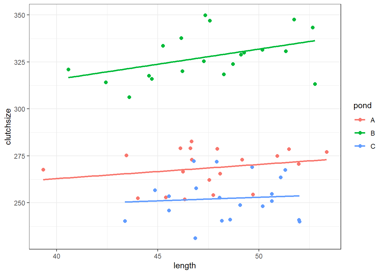
lm_golden <- lm(clutchsize ~ length*pond, goldentoad)
summary(lm_golden)
Call:
lm(formula = clutchsize ~ length * pond, data = goldentoad)
Residuals:
Min 1Q Median 3Q Max
-23.0456 -6.6815 -0.8263 7.7179 22.2570
Coefficients:
Estimate Std. Error t value Pr(>|t|)
(Intercept) 232.7146 38.6258 6.025 1.56e-07 ***
length 0.7550 0.8125 0.929 0.357
pondB 18.6008 53.4338 0.348 0.729
pondC 1.2410 63.8124 0.019 0.985
length:pondB 0.8565 1.1233 0.762 0.449
length:pondC -0.3744 1.3252 -0.283 0.779
---
Signif. codes: 0 '***' 0.001 '**' 0.01 '*' 0.05 '.' 0.1 ' ' 1
Residual standard error: 11.4 on 54 degrees of freedom
Multiple R-squared: 0.9009, Adjusted R-squared: 0.8917
F-statistic: 98.18 on 5 and 54 DF, p-value: < 2.2e-16We’re going to use the seaborn package here, instead of just matlibplot, for efficiency.
(If you’d prefer, however, you can just use plotnine and copy the R code from the other tab.)
plt.clf()
sns.lmplot(data=goldentoad, x="length", y="clutchsize", hue="pond", height=5, aspect=1.3,
scatter_kws={"s": 40}, line_kws={"linewidth": 2}, ci=None)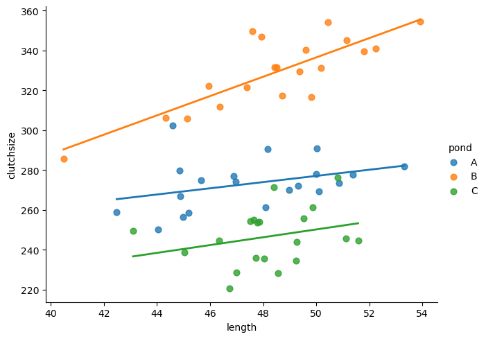
plt.grid(True)
plt.show()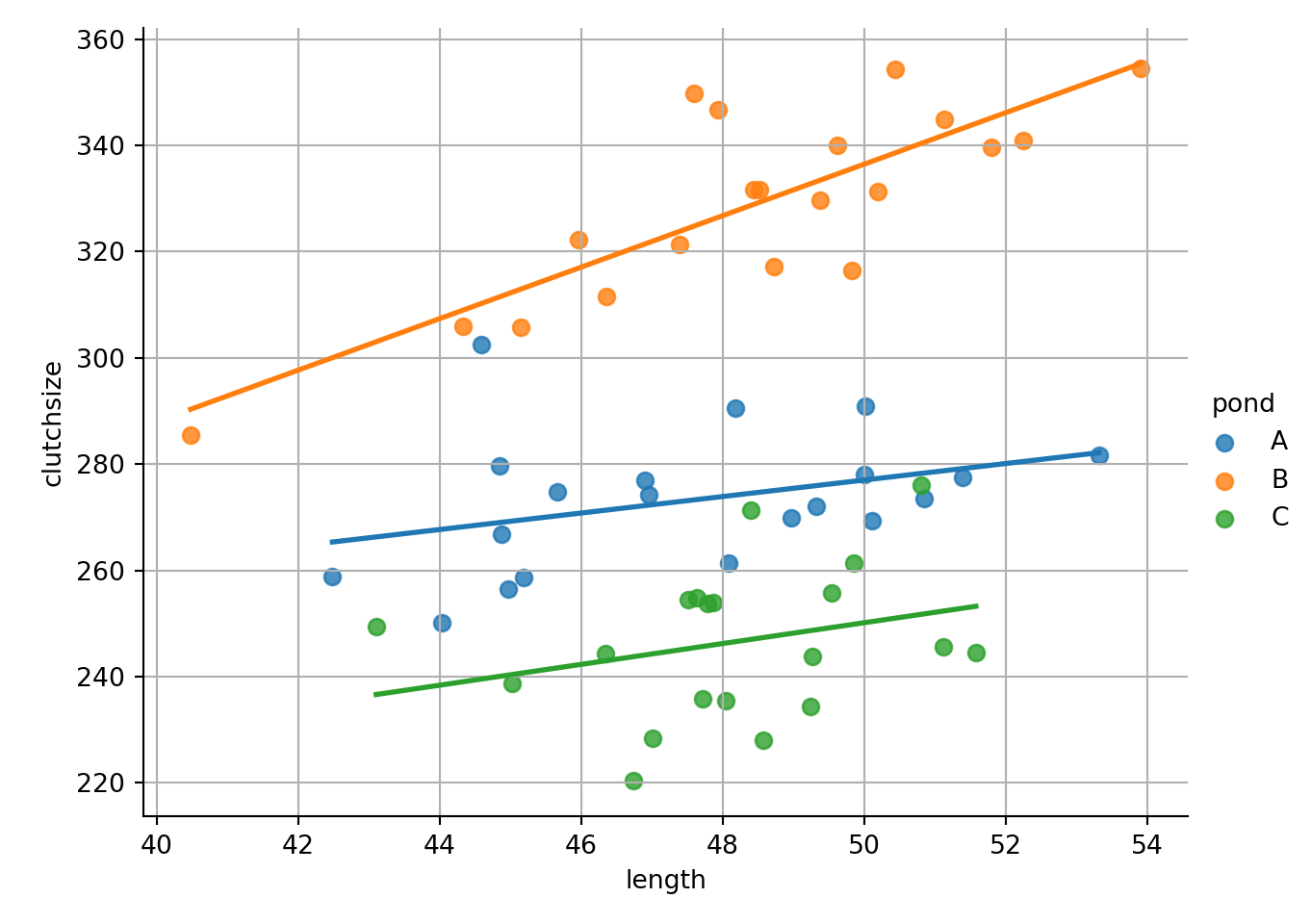

model = smf.ols(formula= "clutchsize ~ length * pond", data = goldentoad)

lm_golden = model.fit()
print(lm_golden.summary())
OLS Regression Results
==============================================================================
Dep. Variable: clutchsize R-squared: 0.900
Model: OLS Adj. R-squared: 0.891
Method: Least Squares F-statistic: 97.36
Date: Mon, 16 Mar 2026 Prob (F-statistic): 9.33e-26
Time: 17:26:54 Log-Likelihood: -233.42
No. Observations: 60 AIC: 478.8
Df Residuals: 54 BIC: 491.4
Df Model: 5
Covariance Type: nonrobust
====================================================================================
coef std err t P>|t| [0.025 0.975]
------------------------------------------------------------------------------------
Intercept 199.3514 46.822 4.258 0.000 105.480 293.223
pond[T.B] -105.3064 65.251 -1.614 0.112 -236.126 25.513
pond[T.C] -47.2483 82.637 -0.572 0.570 -212.925 118.428
length 1.5531 0.983 1.580 0.120 -0.418 3.524
length:pond[T.B] 3.2955 1.357 2.428 0.019 0.574 6.017
length:pond[T.C] 0.4078 1.721 0.237 0.814 -3.043 3.859
==============================================================================
Omnibus: 4.125 Durbin-Watson: 2.550
Prob(Omnibus): 0.127 Jarque-Bera (JB): 3.455
Skew: 0.582 Prob(JB): 0.178
Kurtosis: 3.166 Cond. No. 3.23e+03
==============================================================================
Notes:
[1] Standard Errors assume that the covariance matrix of the errors is correctly specified.
[2] The condition number is large, 3.23e+03. This might indicate that there are
strong multicollinearity or other numerical problems.We can see that we get three separate lines of best fit, with different gradients and intercepts.
How do these map onto our beta coefficients?
- The intercept and gradient for pond
Aare captured inb0andb1 - The differences between the intercept of pond
Aand the intercepts of pondsBandCare captured inb2 - The differences in gradients between pond
Aand the gradients of pondsBandCare captured inb3
Ultimately, there are still 6 unique numbers; but, because of the format of the equation of a linear model, they’re split across 4 separate beta coefficients.
9.4 Two categorical predictors
Last but not least: what happens if we have an interaction between two categorical predictors?
We’ll use a binary predictor variable, presence of predators (yes/no), as our second categorical predictor alongside pond.
Set up parameters and predictors
By now, most of this should look familiar. We construct predators just like we do pond, by repeating the elements of a list/vector.
(To keep things simple, we’ll drop our continuous length predictor for this example.)
rm(list=ls()) # optional clean-up

set.seed(20)

n <- 60
b0 <- 165
b1 <- c(0, 30, -10)   # pond (A, B, C)
b2 <- c(0, 20)        # presence of predator (no, yes)

sdi <- 20

length <- rnorm(n, 48, 3)
pond <- rep(c("A", "B", "C"), each = n/3)

predators <- rep(c("yes", "no"), times = n/2)del(length, pond, goldentoad, clutchsize, avg_clutch) # optional clean-upnp.random.seed(23)
n = 60
b0 = 165
b1 = np.array([0, 30, -10]) # pond (A, B, C)
b2 = np.array([0, 20]) # presence of predator (no, yes)
sdi = 20
length = np.random.normal(48, 3, n)
pond = np.repeat(["A","B","C"], repeats = n//3)
predators = np.tile(["yes","no"], reps = n//2)You’ll notice that we haven’t specified b3 yet - the next section is dedicated to this, since it gets a bit abstract.
The interaction coefficient
What on earth does our b3 coefficient need to look like?
Well, we know it needs to be a vector. Any interaction that contains at least one categorical predictor, requires a vector beta coefficient.
Let’s look at the design matrix for the pond:predators interaction to help us figure that out.
model.matrix(~0 + pond:predators) pondA:predatorsno pondB:predatorsno pondC:predatorsno pondA:predatorsyes
1 0 0 0 1
2 1 0 0 0
3 0 0 0 1
4 1 0 0 0
5 0 0 0 1
6 1 0 0 0
pondB:predatorsyes pondC:predatorsyes
1 0 0
2 0 0
3 0 0
4 0 0
5 0 0
6 0 0Xpond_pred = dmatrix('0 + C(pond):C(predators)', data = {'pond': pond, 'predators': predators})array([[0., 0., 0., 1., 0., 0.],
[1., 0., 0., 0., 0., 0.],
[0., 0., 0., 1., 0., 0.],
[1., 0., 0., 0., 0., 0.],
[0., 0., 0., 1., 0., 0.]])The matrix is 60 rows long (here we’re looking at just the top few rows) and has 6 columns.
Those 6 columns represent our 6 possible subgroups, telling us that our b4 coefficient will need to be 6 elements long. Some of these elements will be 0s, but how many?
The short answer is this:
The first 4 elements will be 0s, because our b0, b1 and b2 coefficients already contain values for 4 of our subgroups. We then need two additional unique numbers for the remaining 2 subgroups.
TipFor a longer answer:
Remember that when fitting the model, our software will choose a group as a reference group.
In this example, b0 is the mean of our reference group, which here is pondA:predatorsno (determined alphabetically).
Our other beta coefficients then represent the differences between this reference group mean, and our other group means.
b0, the baseline mean of our reference grouppondA:predatorsnob2, containing two numbers; these capture the difference between the reference group andpondB:predatorsno/pondC:predatorsnob3, containing one number; this captures the difference between the reference group andpondA:predatorsyes
If we didn’t include a b3 at all, we would get a dataset that looks like this:
`summarise()` has grouped output by 'pond'. You can override using the
`.groups` argument.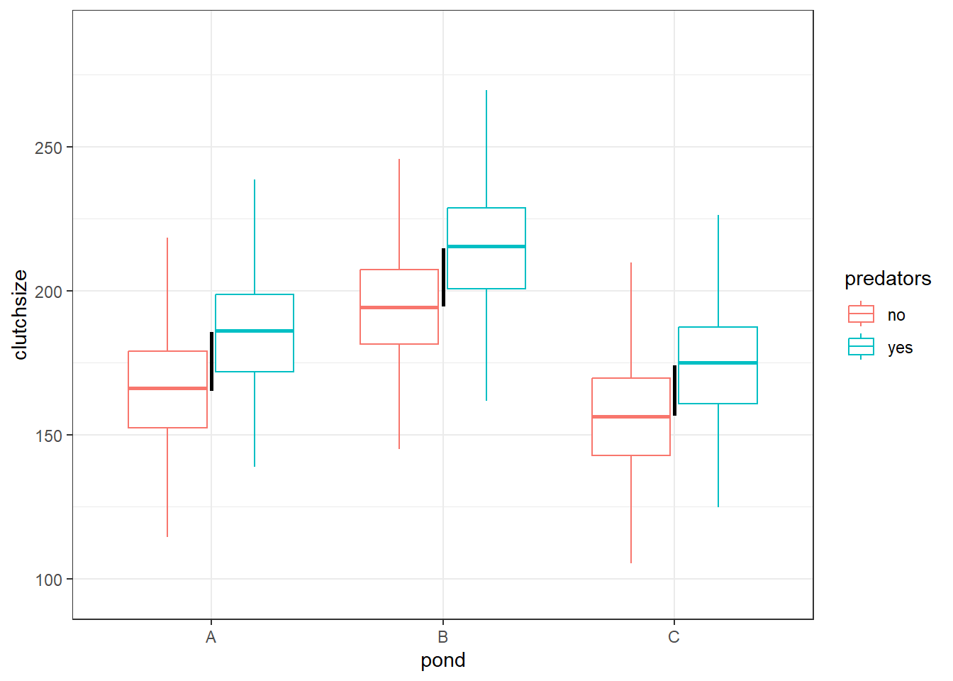
Here, the difference in group means between pondA:predatorsno and pondA:predatorsyes is the exact same difference as we see within ponds B and C as well. That’s represented by the black lines, which are all identical in height.
This means that the only information we need to recreate the 6 group means is the 4 values from our b0, b1 and b2 coefficients.
If we include the interaction term, however, then that’s no longer the case. Within each pond, there can be a completely unique difference between when predators were and weren’t present:
`summarise()` has grouped output by 'pond'. You can override using the
`.groups` argument.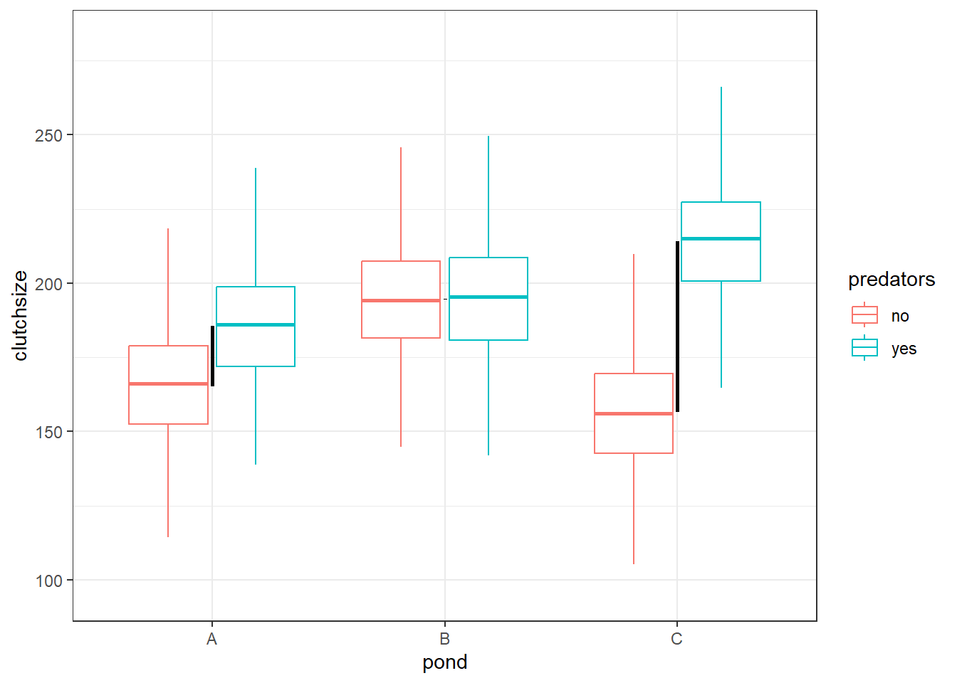
Now, we cannot use the same b2 value (yes vs no predators) for each of our three ponds: we need unique differences.
Or, to phrase it another way: each of our 5 non-reference subgroups will have a completely unique difference in means from our reference subgroup.
This means our simulation needs to provide 6 unique values across our beta coefficients. We already have the first 4, from b0, b1 and b2, so we just need two more.
This, therefore, is what our b3 looks like:
b3 <- c(0, 0, 0, 0, -20, 40)b3 = np.array([0, 0, 0, 0, -20, 40])Since there are 6 subgroups, and the first 4 from our model design matrix are already dealt with, we only need two additional numbers. The other groups don’t need to be adjusted further.
Simulate response variable & check dataset
Finally, we simulate our response variable, and then we can check how well our model does at recovering these parameters.
b3 <- c(0, 0, 0, 0, -20, 40)    # interaction pond:predators

avg_clutch <- b0 + model.matrix(~0+pond) %*% b1 + model.matrix(~0+predators) %*% b2 + model.matrix(~0+pond:predators) %*% b3
clutchsize <- rnorm(n, avg_clutch, sdi)

toads <- tibble(clutchsize, length, pond, predators)

# fit and summarise model
lm_toads <- lm(clutchsize ~ length + pond * predators, toads)
summary(lm_toads)
Call:
lm(formula = clutchsize ~ length + pond * predators, data = toads)

Residuals:
    Min      1Q  Median      3Q     Max
-34.890 -11.348  -0.284   9.929  37.223

Coefficients:
                   Estimate Std. Error t value Pr(>|t|)
(Intercept)        241.8247    37.8165   6.395 4.24e-08 ***
length              -1.8881     0.7868  -2.400   0.0200 *
pondB               48.0543     8.0604   5.962 2.08e-07 ***
pondC                2.5931     8.0643   0.322   0.7491
predatorsyes        40.9971     8.0570   5.088 4.86e-06 ***
pondB:predatorsyes -37.6927    11.4020  -3.306   0.0017 **
pondC:predatorsyes  23.7371    11.4269   2.077   0.0426 *
---
Signif. codes:  0 '***' 0.001 '**' 0.01 '*' 0.05 '.' 0.1 ' ' 1

Residual standard error: 18.01 on 53 degrees of freedom
Multiple R-squared:  0.693, Adjusted R-squared:  0.6583
F-statistic: 19.94 on 6 and 53 DF,  p-value: 4.978e-12
b3 = np.array([0, 0, 0, 0, -20, 40]) # interaction pond:predators
# construct design matrices
Xpond = dmatrix('0 + C(pond)', data = {'pond': pond})
Xpred = dmatrix('0 + C(predators)', data = {'predators': predators})
Xpond_pred = dmatrix('0 + C(pond):C(predators)', data = {'pond': pond, 'predators': predators})
# simulate response variable in two steps
avg_clutch = b0 + np.dot(Xpond, b1) + np.dot(Xpred, b2) + np.dot(Xpond_pred, b3)
clutchsize = np.random.normal(avg_clutch, sdi, n)
# collate dataset
goldentoad = pd.DataFrame({'pond': pond, 'length': length, 'clutchsize': clutchsize})
# fit and summarise model
model = smf.ols(formula= "clutchsize ~ pond * predators", data = goldentoad)
lm_golden = model.fit()
print(lm_golden.summary()) OLS Regression Results
==============================================================================
Dep. Variable: clutchsize R-squared: 0.473
Model: OLS Adj. R-squared: 0.425
Method: Least Squares F-statistic: 9.704
Date: Mon, 16 Mar 2026 Prob (F-statistic): 1.19e-06
Time: 17:26:57 Log-Likelihood: -265.96
No. Observations: 60 AIC: 543.9
Df Residuals: 54 BIC: 556.5
Df Model: 5
Covariance Type: nonrobust
==============================================================================================
coef std err t P>|t| [0.025 0.975]
----------------------------------------------------------------------------------------------
Intercept 174.9817 6.787 25.781 0.000 161.374 188.589
pond[T.B] 30.7008 9.599 3.198 0.002 11.457 49.945
pond[T.C] -25.7779 9.599 -2.686 0.010 -45.022 -6.534
predators[T.yes] 10.4013 9.599 1.084 0.283 -8.843 29.646
pond[T.B]:predators[T.yes] -22.1565 13.575 -1.632 0.108 -49.372 5.059
pond[T.C]:predators[T.yes] 44.0281 13.575 3.243 0.002 16.813 71.244
==============================================================================
Omnibus: 1.332 Durbin-Watson: 2.384
Prob(Omnibus): 0.514 Jarque-Bera (JB): 1.357
Skew: 0.325 Prob(JB): 0.507
Kurtosis: 2.652 Cond. No. 9.77
==============================================================================
Notes:
[1] Standard Errors assume that the covariance matrix of the errors is correctly specified.9.5 Three-way interactions
Three-way interactions are rarer than two-way interactions, at least in practice, because they require a much bigger sample size to detect and are harder to interpret.
However, they can occur, so let’s (briefly) look at how you’d simulate them.
length:temperature:pond
This three-way interaction involves two continuous (length and temperature) and one categorical (pond) predictors.
It will, by default, need a vector beta coefficient.
set.seed(22)

n <- 120
b0 <- -30               # intercept
b1 <- 0.7               # main effect of length
b2 <- c(0, 30, -10)     # main effect of pond
b3 <- 0.5               # main effect of temperature

b4 <- 0.25              # interaction of length:temperature
b5 <- c(0, 0.2, -0.1)   # interaction of length:pond
b6 <- c(0, 0.1, -0.25)  # interaction of temperature:pond

b7 <- c(0, 0.05, -0.1)  # interaction of length:temp:pond

sdi <- 6np.random.seed(28)
n = 120
b0 = -30 # intercept
b1 = 0.7 # main effect of length
b2 = np.array([0, 30, -10]) # main effect of pond
b3 = 0.5 # main effect of temperature
b4 = 0.25 # interaction of length:temperature
b5 = np.array([0, 0.2, -0.1]) # interaction of length:pond
b6 = np.array([0, 0.1, -0.25]) # interaction of temperature:pond
b7 = np.array([0, 0.05, -0.1]) # interaction of length:temp:pond
sdi = 6There are 12 unique/non-zero values across our 8 beta coefficients.
One helpful way to think about this: within each pond, we need 4 unique numbers/constants to describe the intercept, main effect of length, main effect of temperature, and two-way interaction between length:temperature.
Since we’re allowing a three-way interaction, each of the three ponds will (or at least, can) have a completely unique set of 4 values.
# generate predictor variables
length <- rnorm(n, 48, 3)
pond <- rep(c("A", "B", "C"), each = n/3)
temperature <- runif(n, 10, 32)

# generate response variable in two steps
avg_clutch <- b0 + b1*length + model.matrix(~0+pond) %*% b2 + b3*temperature +
  b4*length*temperature +
  model.matrix(~0+length:pond) %*% b5 +
  model.matrix(~0+temperature:pond) %*% b6 +
  model.matrix(~0+length:temperature:pond) %*% b7
clutchsize <- rnorm(n, avg_clutch, sdi)

# collate the dataset
goldentoad <- tibble(length, pond, temperature, clutchsize)
# generate predictor variables
length = np.random.normal(48, 3, n)
pond = np.repeat(["A","B","C"], repeats = n//3)
temperature = np.random.uniform(10, 32, n)
# create design matrices
Xpond = dmatrix('0 + C(pond)', data = {'pond': pond})
Xpond_length = dmatrix('0 + C(pond):length', data = {'pond': pond, 'length': length})
Xpond_temp = dmatrix('0 + C(pond):temp', data = {'pond': pond, 'temp': temperature})
Xpond_temp_length = dmatrix('0 + C(pond):length:temp', data = {'pond': pond, 'length': length, 'temp': temperature})
# generate response variable in two steps
avg_clutch = (
b0 + b1*length + np.dot(Xpond, b2) + b3*temperature
+ b4*length*temperature + np.dot(Xpond_length, b5)
+ np.dot(Xpond_temp, b6) + np.dot(Xpond_temp_length, b7)
)
clutchsize = np.random.normal(avg_clutch, sdi, n)
# collate the dataset
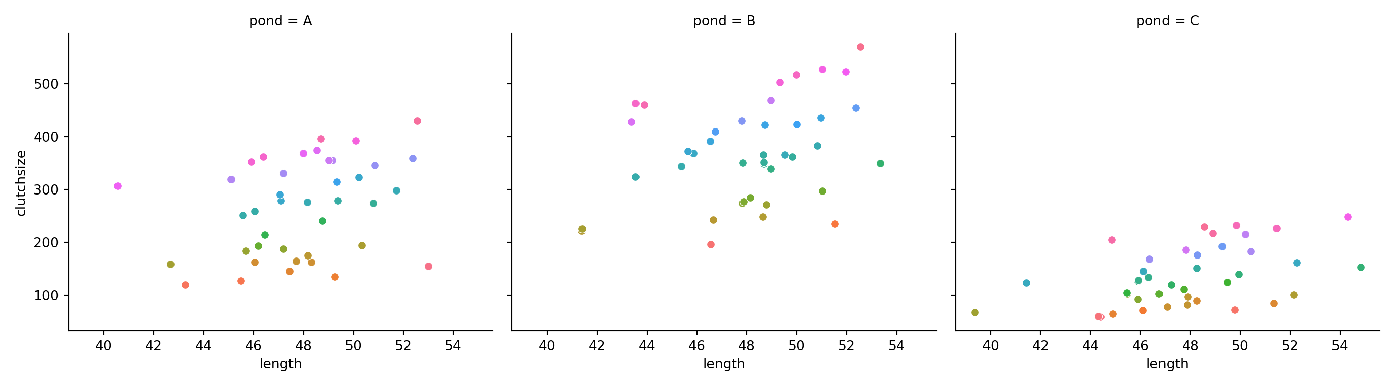
goldentoad = pd.DataFrame({'pond': pond, 'length': length, 'temperature': temperature, 'clutchsize': clutchsize})Let’s check whether these data look sensible by visualising them, and how well a linear model does at recovering the parameters:
ggplot(goldentoad, aes(x = length, colour = temperature, y = clutchsize)) +
  facet_wrap(~ pond) +
  geom_point()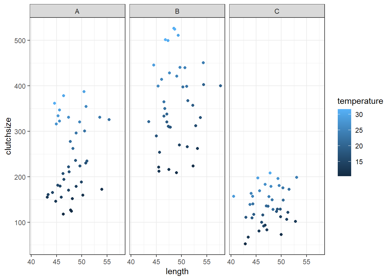
lm_golden <- lm(clutchsize ~ length * pond * temperature, data = goldentoad)
summary(lm_golden)
Call:
lm(formula = clutchsize ~ length * pond * temperature, data = goldentoad)

Residuals:
     Min       1Q   Median       3Q      Max
-20.6864  -4.4287  -0.0933   4.2699  17.4106

Coefficients:
                          Estimate Std. Error t value Pr(>|t|)
(Intercept)              -33.44912   59.94099  -0.558 0.577976
length                     0.64795    1.26547   0.512 0.609683
pondB                     26.82304   94.49979   0.284 0.777075
pondC                    -58.61716   84.66914  -0.692 0.490230
temperature                0.63337    2.98100   0.212 0.832142
length:pondB               0.31095    1.96551   0.158 0.874591
length:pondC               1.15449    1.79169   0.644 0.520711
length:temperature         0.25152    0.06296   3.995 0.000119 ***
pondB:temperature         -0.67053    4.73427  -0.142 0.887633
pondC:temperature          0.84409    4.13926   0.204 0.838798
length:pondB:temperature   0.06567    0.09875   0.665 0.507463
length:pondC:temperature  -0.13405    0.08779  -1.527 0.129706
---
Signif. codes:  0 '***' 0.001 '**' 0.01 '*' 0.05 '.' 0.1 ' ' 1

Residual standard error: 6.51 on 108 degrees of freedom
Multiple R-squared:  0.9972,    Adjusted R-squared:  0.9969
F-statistic:  3534 on 11 and 108 DF,  p-value: < 2.2e-16
We’ll use seaborn to create the faceted plot (though, as always, if you’re used to ggplot/plotnine, you can toggle over to the R code and use that as a basis instead):
plt.clf()
g = sns.FacetGrid(goldentoad, col="pond", hue="temperature", height=4, aspect=1.2)
g.map_dataframe(sns.scatterplot, x="length", y="clutchsize")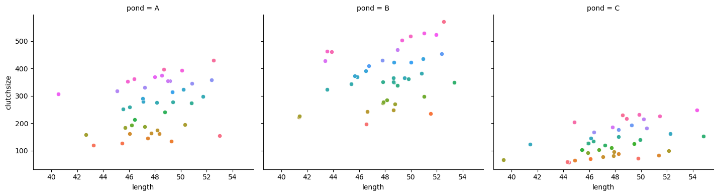
And let’s fit and summarise the model:
model = smf.ols(formula= "clutchsize ~ length * pond * temperature", data = goldentoad)

lm_golden = model.fit()
print(lm_golden.summary())
OLS Regression Results
==============================================================================
Dep. Variable: clutchsize R-squared: 0.998
Model: OLS Adj. R-squared: 0.998
Method: Least Squares F-statistic: 5432.
Date: Mon, 16 Mar 2026 Prob (F-statistic): 1.02e-142
Time: 17:27:04 Log-Likelihood: -370.91
No. Observations: 120 AIC: 765.8
Df Residuals: 108 BIC: 799.3
Df Model: 11
Covariance Type: nonrobust
================================================================================================
coef std err t P>|t| [0.025 0.975]
------------------------------------------------------------------------------------------------
Intercept -66.5326 48.314 -1.377 0.171 -162.299 29.233
pond[T.B] 107.8100 68.883 1.565 0.120 -28.729 244.349
pond[T.C] 48.7665 67.082 0.727 0.469 -84.202 181.735
length 1.4876 1.014 1.467 0.145 -0.523 3.498
length:pond[T.B] -1.5205 1.443 -1.054 0.294 -4.381 1.340
length:pond[T.C] -1.3506 1.407 -0.960 0.339 -4.139 1.438
temperature 0.6124 2.123 0.288 0.774 -3.596 4.821
pond[T.B]:temperature -0.9611 3.030 -0.317 0.752 -6.966 5.044
pond[T.C]:temperature -1.9374 3.148 -0.615 0.540 -8.177 4.302
length:temperature 0.2466 0.044 5.556 0.000 0.159 0.335
length:pond[T.B]:temperature 0.0769 0.063 1.216 0.227 -0.048 0.202
length:pond[T.C]:temperature -0.0646 0.065 -0.987 0.326 -0.194 0.065
==============================================================================
Omnibus: 2.940 Durbin-Watson: 2.011
Prob(Omnibus): 0.230 Jarque-Bera (JB): 2.966
Skew: 0.065 Prob(JB): 0.227
Kurtosis: 3.759 Cond. No. 2.14e+05
==============================================================================
Notes:
[1] Standard Errors assume that the covariance matrix of the errors is correctly specified.
[2] The condition number is large, 2.14e+05. This might indicate that there are
strong multicollinearity or other numerical problems.
Try fitting a purely additive model. Better or worse?
length:pond:predators
Now, let’s look at a three-way interaction that contains two categorical predictors.
Within each pond, there are 4 key numbers that we need:
- The intercept for the
predatorreference group - The
lengthgradient for thepredatorreference group - The adjustment to the intercept for the
predatornon-reference group - The adjustment the
lengthgradient for thepredatornon-reference group
(It can really help to draw this out on some scrap paper!)
So, across our 8 beta coefficients, we’re going to need 12 numbers.
set.seed(22)

n <- 120
b0 <- -30                         # intercept
b1 <- 0.7                         # main effect of length
b2 <- c(0, 30, -10)               # main effect of pond (A, B, C)
b3 <- c(0, 20)                    # main effect of predators (no, yes)

b4 <- c(0, 0.2, -0.1)             # interaction of length:pond
b5 <- c(0, 0.1)                   # interaction of length:predators
b6 <- c(0, 0, 0, 0, 0.1, -0.25)   # interaction of pond:predators

b7 <- c(0, 0, 0, 0, 0.1, -0.2)    # interaction of length:temp:pond

sdi <- 6np.random.seed(28)
n = 120
b0 = -30 # intercept
b1 = 0.7 # main effect of length
b2 = np.array([0, 30, -10]) # main effect of pond (A, B, C)
b3 = np.array([0, 20]) # main effect of predators (no, yes)
b4 = np.array([0, 0.2, -0.1]) # interaction of length:pond
b5 = np.array([0, 0.1]) # interaction of length:predators
b6 = np.array([0, 0, 0, 0, 0.1, -0.25]) # interaction of pond:predators
b7 = np.array([0, 0, 0, 0, 0.1, -0.2]) # interaction of length:temp:pond
sdi = 6If you’re curious how we were supposed to know to put all the leading zeroes in our b6 and b7 coefficients - the answer is, by looking ahead and checking the number of columns in the design matrix!
# generate predictor variables
length <- rnorm(n, 48, 3)
pond <- rep(c("A", "B", "C"), each = n/3)
predators <- rep(c("yes", "no"), times = n/2)

# generate response variable
avg_clutch <- b0 + b1*length + model.matrix(~0+pond) %*% b2 + model.matrix(~0+predators) %*% b3 +
  model.matrix(~0+length:pond) %*% b4 +
  model.matrix(~0+length:predators) %*% b5 +
  model.matrix(~0+pond:predators) %*% b6 +
  model.matrix(~0+length:pond:predators) %*% b7
clutchsize <- rnorm(n, avg_clutch, sdi)

# collate the dataset
goldentoad <- tibble(length, pond, predators, clutchsize)
# generate predictor variables
length = np.random.normal(48, 3, n)
pond = np.repeat(["A","B","C"], repeats = n//3)
predators = np.tile(["yes","no"], reps = n//2)
# create design matrices
Xpond = dmatrix('0 + C(pond)', data = {'pond': pond})
Xpred = dmatrix('0 + C(pred)', data = {'pred': predators})
Xpond_length = dmatrix('0 + C(pond):length', data = {'pond': pond, 'length': length})
Xlength_pred = dmatrix('0 + length:C(pred)', data = {'pred': predators, 'length': length})
Xpond_pred = dmatrix('0 + C(pond):C(pred)', data = {'pond': pond, 'pred': predators})
Xpond_length_pred = dmatrix('0 + length:C(pond):C(pred)', data = {'pond': pond, 'length': length, 'pred': predators})
# generate response variable in two steps
avg_clutch = (
b0 + b1*length + np.dot(Xpond, b2) + np.dot(Xpred, b3)
+ np.dot(Xpond_length, b4) + np.dot(Xlength_pred, b5)
+ np.dot(Xpond_pred, b6) + np.dot(Xpond_length_pred, b7)
)
clutchsize = np.random.normal(avg_clutch, sdi, n)
# collate the dataset
goldentoad = pd.DataFrame({'pond': pond, 'length': length, 'temperature': temperature, 'clutchsize': clutchsize})9.6 Exercises
9.6.1 Continuing your own simulation
9.7 Summary
Once we know how to simulate main effects, the main additional challenge for simulating interactions is to think about what the beta coefficients should look like (especially when a categorical predictor is involved).
Visualising the dataset repeatedly, and going back to tweak the parameters, is often necessary when trying to simulate an interaction.
TipKey Points
- Interactions containing only continuous predictors, only require a single constant as their beta coefficient
- While any interaction term containing a categorical predictor, must also be treated as categorical when simulating
- It’s very helpful to visualise the dataset to check your simulation is as expected