library(tidyverse)
library(rstatix)6 Confidence intervals
In this chapter, we’ll use simulation to answer the deceptively simple question: what are confidence intervals, and how should they be interpreted?
6.1 Libraries and functions
NoteClick to expand
import pandas as pd
import numpy as np
import random
import statistics
import matplotlib.pyplot as plt
import statsmodels.stats.api as sms
from scipy.stats import t
Confidence intervals, like p-values, are misunderstood surprisingly often in applied statistics. It’s understandable that this happens, because a single set of confidence intervals by itself might not mean very much, unless you understand more broadly where they come from.
Simulation is a fantastic way to gain this understanding.
6.2 Extracting confidence intervals for a single sample
Let’s start by showing how we can calculate confidence intervals from just one dataset.
We’re still using one-dimensional data, so our confidence intervals in this case are for the mean.
Method 1
Method 1 in R uses the t.test function. This is simpler in our current one-dimensional situation.
The confidence intervals are a standard part of the t-test, and we can use the $ syntax to extract them specifically from the output:
set.seed(21)

n <- 40
mean_n <- 6
sd_n <- 1.5

data <- rnorm(n, mean_n, sd_n)

conf.int <- t.test(data, conf.level = 0.95)$conf.int

print(conf.int)
[1] 5.647455 6.678777
attr(,"conf.level")
[1] 0.95Method 2
Method 2 in R is via the confint function, which takes an lm object as its first argument.
We’ve had to do a bit of extra work to be able to use the lm function in this case (making our data into a dataframe), but in future sections of the course where we simulate multi-dimensional data, we’ll have to do this step anyway - so this method may work out more efficient later on.
set.seed(21)

n <- 40
mean_n <- 6
sd_n <- 1.5

data <- rnorm(n, mean_n, sd_n) %>%
  data.frame()

lm_data <- lm(. ~ 1, data)

confint(lm_data, level = 0.95)
2.5 % 97.5 %
(Intercept) 5.647455 6.678777There are a few options for extracting confidence intervals in Python, but perhaps the most efficient is via statsmodels.stats.api:
np.random.seed(20)

n = 40
mean = 6
sd = 1.5

data = np.random.normal(mean, sd, n)

sms.DescrStatsW(data).tconfint_mean()
(5.241512557961966, 6.341197862942866)6.3 Extracting multiple sets of confidence intervals
Now, let’s use a for loop to extract and save multiple sets of confidence intervals.
We’ll stick to the same parameters we used above:
set.seed(21)

# Soft-code the number of iterations
iterations <- 100

# Soft-code the simulation parameters
n <- 40
mean_n <- 6
sd_n <- 1.5

# Initialise a dataframe to store the results of the iterations
intervals <- data.frame(mean = numeric(iterations),
                        lower = numeric(iterations),
                        upper = numeric(iterations))

# Run simulations
for (i in 1:iterations) {

  data <- rnorm(n, mean_n, sd_n) %>%
    data.frame()

  lm_data <- lm(. ~ 1, data)

  # Extract mean and confidence intervals as simple numeric objects
  est_mean <- unname(coefficients(lm_data)[1])
  est_lower <- confint(lm_data, level = 0.95)[1]
  est_upper <- confint(lm_data, level = 0.95)[2]

  # Update appropriate row of empty intervals object, with values from this loop
  intervals[i,] <- data.frame(mean = est_mean, lower = est_lower, upper = est_upper)

}

head(intervals)
mean lower upper
1 6.163116 5.647455 6.678777
2 6.112842 5.601488 6.624196
3 5.771928 5.313615 6.230240
4 5.926402 5.489371 6.363432
5 5.916349 5.481679 6.351019
6 6.180240 5.742182 6.618298np.random.seed(30)
iterations = 100
n = 40
mean = 6
sd = 1.5
rows = []
for i in range(iterations):
data = np.random.normal(mean, sd, n)
estmean = statistics.mean(data)
lower = sms.DescrStatsW(data).tconfint_mean()[0]
upper = sms.DescrStatsW(data).tconfint_mean()[1]
rows.append({'mean': estmean, 'lower': lower, 'upper': upper})
intervals = pd.DataFrame(rows)
intervals.head() mean lower upper
0 5.787213 5.223520 6.350906
1 5.760226 5.256582 6.263870
2 6.176261 5.716103 6.636418
3 6.214928 5.795727 6.634128
4 5.988544 5.452712 6.524377Just by looking at the first few sets of intervals, we can see - as expected - that our set of estimated means are varying around the true population value (in an approximately normal manner, according to the central limit theorem, as we now know).
We can also see that our confidence intervals are approximately following the mean estimate in each case. When the mean estimate is a bit high or a bit low relative to the true value, our confidence intervals are shifted up or down a bit, such that the estimated mean sits in the middle of the confidence intervals for each individual dataset.
In other words: each confidence interval is a property of its dataset.
To get a clearer picture, let’s visualise them:
intervals %>%
  ggplot(aes(x = 1:iterations)) +
    geom_point(aes(y = mean)) +
    geom_segment(aes(y = lower, yend = upper)) +
    geom_hline(yintercept = mean_n, colour = "red")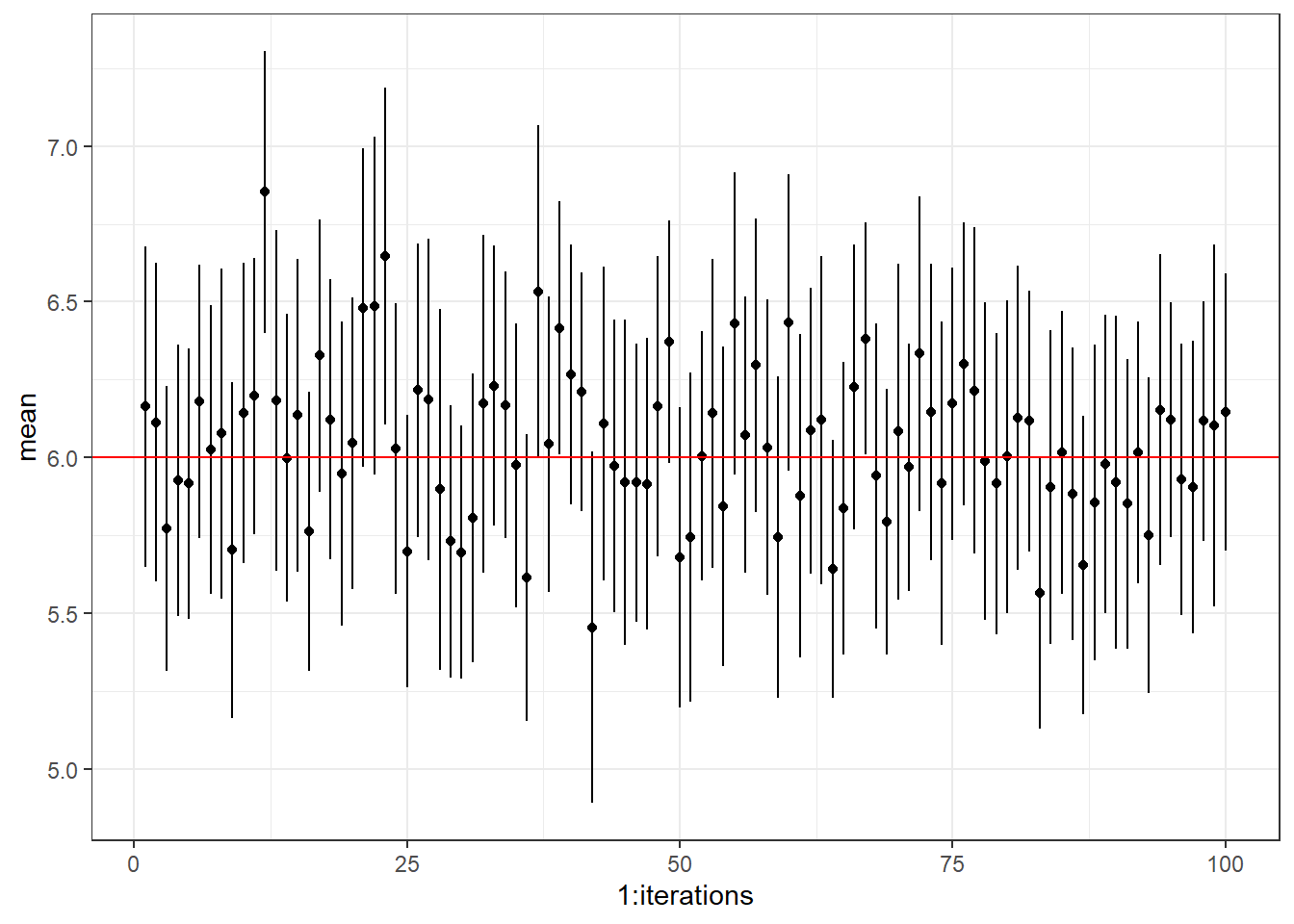
fig, ax = plt.subplots(figsize=(8, 6))

for i in range(iterations):
    ax.plot([i + 1, i + 1], [intervals['lower'][i], intervals['upper'][i]], color='black')
    ax.plot(i + 1, intervals['mean'][i], 'o', color='black')

ax.axhline(y=mean, color='red', linestyle='--', label='True Mean')

plt.show()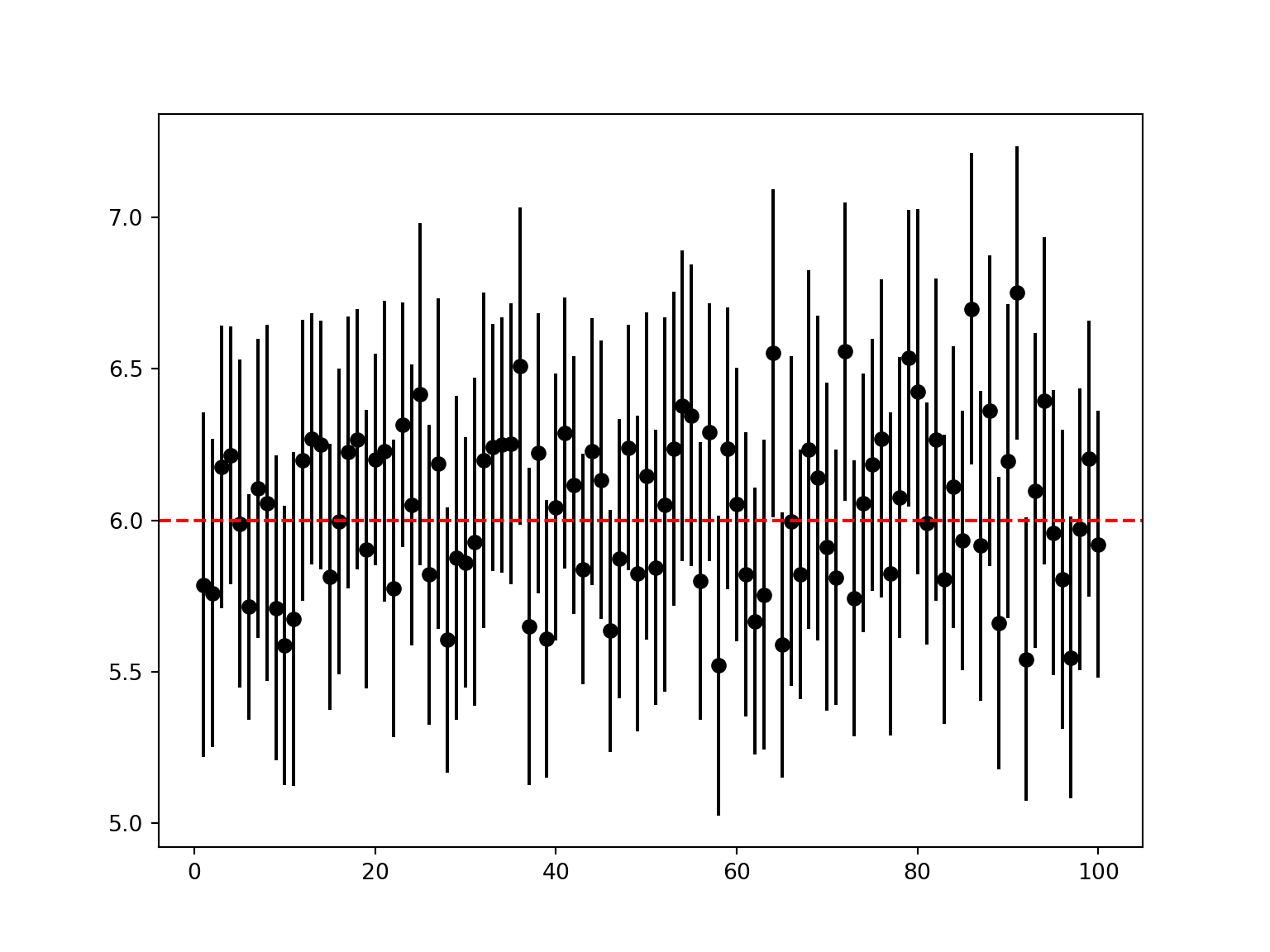
From this plot, with the true population mean overlaid, we can see that most of the confidence intervals are managing to capture that true value. But a small proportion aren’t.
What proportion of the intervals are managing to capture the true population mean?
We can check like so:
mean(mean_n <= intervals$upper & mean_n >= intervals$lower)[1] 0.95contains_true = (intervals['lower'] <= mean) & (intervals['upper'] >= mean)
contains_true.mean()0.95Given that we set our confidence intervals at the 95% level, this is exactly what the simulation should reveal: approximately (in this case, exactly) 95 of our 100 confidence intervals contain the true population mean.
WarningThe confidence is about the intervals, not the parameter
The very definition of 95% confidence intervals is this: we expect that the confidence intervals from 95% of the samples drawn from a given population with a certain parameter, to contain that true population parameter.
This is not equivalent to saying that there is a 95% chance that the true population value falls inside a given interval. This is a common misconception, but there is no probability associated with the true population value - it just is what it is (even if we don’t know it).
As with p-values, the probability is associated with datasets/samples when talking about confidence intervals, not with the underlying population.
TipCalculating confidence intervals manually
For those of you who are curious about the underlying mathematical formulae for confidence intervals, and how to calculate them manually, it’s done like so:
- Calculate the sample mean
- Calculate the (estimated) standard error of the mean
- Find the t-score* that corresponds to the confidence level (e.g., 95%)
- Calculate the margin of error and construct the confidence interval
*You can use z-scores, but t-scores tend to be more appropriate for small samples.
Let’s start by simulating a simple dataset.
set.seed(21)

n <- 40
mean_n <- 6
sd_n <- 1.5

data <- rnorm(n, mean_n, sd_n)
Step 1: Calculate the sample mean
sample_mean <- mean(data)
print(sample_mean)
[1] 6.163116Step 2: Calculate the standard error of the mean
We do this by dividing the sample standard deviation by the square root of the sample size, \(\frac{s}{\sqrt{N}}\).
sample_se <- sd(data)/sqrt(n)
print(sample_se)
[1] 0.2549382Step 3: Calculate the t-score corresponding to the confidence level
This step also gives a clue as to how the significance threshold (or \(\alpha\)) is associated with confidence level (they add together to equal 1).
alpha <- 0.05

sample_df <- n - 1

t_score = qt(p = alpha/2, df = sample_df, lower.tail = FALSE)
print(t_score)
[1] 2.022691Step 4: Calculate the margin of error and construct the confidence interval
# How many standard deviations away from the mean, is the margin of error?
margin_error <- t_score * sample_se

# Calculate upper & lower bounds around the mean
lower_bound <- sample_mean - margin_error
upper_bound <- sample_mean + margin_error

print(c(lower_bound,upper_bound))
[1] 5.647455 6.678777If we compare that to what we would’ve gotten, if we’d used a function to do it for us:
data %>%
  data.frame() %>%
  lm(data = ., formula = . ~ 1, ) %>%
  confint(level = 0.95)
2.5 % 97.5 %
(Intercept) 5.647455 6.678777… we can indeed see that we get exactly the same values.
Let’s start by simulating a simple dataset.
np.random.seed(20)

n = 40
mean = 6
sd = 1.5

data = np.random.normal(mean, sd, n)
Step 1: Calculate the sample mean and standard deviation
sample_mean = np.mean(data)
sample_sd = np.std(data)
print(sample_mean, sample_sd)
5.791355210452416 1.69762282725244Step 2: Calculate the standard error of the mean
We do this by dividing the sample standard deviation by the square root of the sample size, \(\frac{s}{\sqrt{N}}\).
sample_se = sample_sd/np.sqrt(n)
print(sample_se)0.26841773710061373Step 3: Calculate the t-score corresponding to the confidence level
This step also gives a clue as to how the significance threshold (or \(\alpha\)) is associated with confidence level (they add together to equal 1).
from scipy.stats import t

alpha = 0.05
sample_df = n-1

t_crit = t.ppf(1-alpha/2, sample_df)
print(t_crit)2.022690911734728Step 4: Calculate the margin of error and construct the confidence interval
First, we find the margin of error: how many standard deviations away from the mean is our cut-off?
Then, we use that to find the upper and lower bounds, around the mean.
margin_error = t_crit * sample_se

ci = (sample_mean - margin_error, sample_mean + margin_error)

print(ci)
(5.248429093070603, 6.334281327834229)If we compare that to what we would’ve gotten, if we’d used a function to do it for us:
sms.DescrStatsW(data).tconfint_mean()(5.241512557961966, 6.341197862942866)… we can indeed see that we get the same interval, plus or minus some tiny differences in numerical precision from the different functions used.
If you think about things in a maths-ier way, it can be helpful to know how something is calculated - but you will probably always use existing functions when actually coding this stuff!
6.4 Exercises
6.4.1 Width of confidence intervals
There are multiple factors that will affect the width of confidence intervals.
In this exercise, you’ll test some of them, to get an intuition of how (and hopefully why).
6.5 Summary
Confidence intervals are commonly misunderstood, which is really easy to do when you’re only thinking about one dataset.
However, simulation allows us to look at a massive number of datasets that all come from the same underlying population, meaning we can look at multiple sets of confidence intervals - which puts the real interpretation of confidence intervals into context!
TipKey Points
- If you construct 100 sets of 95% confidence intervals, you should expect ~95 of them to contain the true population parameter
- This is not the same as a 95% chance of the true population parameter being contained inside any individual set of confidence intervals
- The probability is associated with the intervals, not with the parameter!