library(tidyverse)
library(rstatix)

# These packages will be used for evaluating the models we fit to our simulated data
library(performance)
library(ggResidpanel)

# This package is optional/will only be used for later sections in this chapter
library(MASS)8 Simulating categorical predictors
This chapter follows on closely from the previous chapter on continuous predictors.
8.1 Libraries and functions
NoteClick to expand
import numpy as np
import pandas as pd
import matplotlib.pyplot as plt

import statsmodels.api as sm
import statsmodels.formula.api as smf

from patsy import dmatrix
8.2 The pond variable
We’re going to stick with our golden toads, and keep the continuous length predictor variable from the previous chapter, so that we can build up the complexity of our dataset gradually between chapters.
To add that complexity, we’re going to imagine that golden toads living in different ponds produce slightly different clutch sizes, and simulate some sensible data on that basis.
Clear previous simulation
You might find it helpful to delete variables/clear the global environment, so that nothing from your previous simulation has an unexpected impact on your new one:
rm(list=ls())del(avg_clutch, clutchsize, goldentoad, length, lm_golden, model, tempdata)(This step is optional!)
Simulating categorical predictors
Categorical predictors are a tiny bit more complex to simulate, as the beta coefficients switch from being constants (gradients) to vectors (representing multiple means).
However, we’re still going to follow the same workflow that we used with continuous predictors in the previous chapter:
- Set parameters (seed, sample size, beta coefficients and standard deviation)
- Generate the values of our predictor variable
- Simulate average values of response variable
- Simulate actual values of response variable
- Check the dataset
8.3 Set parameters
Exactly as we did before, we start by setting key parameters including:
- Seed, for reproducibility
- Sample size
n - Individual standard deviation
sdi - Beta coefficients
We need three betas now, since we’re adding a second predictor.
To generate the beta for pond, we need to specify a vector, instead of a single constant. Let’s keep things relatively simple and stick to just three ponds, which we’ll imaginatively call A, B and C.
Since pond A will be our reference group, our beta does not need to contain any adjustment for that pond, hence the vector starts with a 0. The other two numbers then represent the difference in means between pond A and ponds B and C respectively.
set.seed(20)

n <- 60
b0 <- 175             # intercept
b1 <- 2               # main effect of length
b2 <- c(0, 30, -10)   # main effect of pond

sdi <- 20np.random.seed(20)
n = 60
b0 = 175 # intercept
b1 = 2 # main effect of length
b2 = np.array([0, 30, -10]) # main effect of pond
sdi = 20This means that, in the reality we are creating here, the true mean clutch size for each of our three ponds is 175, 205 (175+30) and 165 (175-10).
8.4 Generate values for predictor variable(s)
Next, we need values for our length and pond predictors.
We already know how to generate length from the previous chapter.
For pond, we’re not going to sample from a distribution, because we need category names instead of numeric values. So, we’ll specify our category names and repeat them as appropriate:
length <- rnorm(n, 48, 3)

pond <- rep(c("A", "B", "C"), each = n/3)
Tiprep and c functions
The rep and c functions in R (c short for concatenate) will come up quite a lot when generating predictor variables.
The rep function takes two arguments each time:
- First, an argument containing the thing that you want repeated (which can either be a single item, or a list/vector)
- Second, an argument containing information about how many times to repeat the first argument (there are actually multiple options for how to phrase this second argument)
The c function is a little simpler: it combines, i.e., concatenates, all of the arguments you put into it into a single vector/list item.
You can then combine these two functions together in various ways to achieve what you want.
For example, these two lines of code both produce the same output:
c(rep("A", times = 3), rep("B", times = 3))[1] "A" "A" "A" "B" "B" "B"rep(c("A", "B"), each = 3)[1] "A" "A" "A" "B" "B" "B"The first version asks for "A" to be repeated 3 times, "B" to be repeated 3 times, and then these two triplets to be concatenated together into one list.
The second version asks us to take a list of two items, "A", "B", and repeat each element 3 times each.
Meanwhile, the code below will do something very different:
rep(c("A", "B"), times = 3)[1] "A" "B" "A" "B" "A" "B"This line of code asks us to take the list "A", "B" and repeat it, as-is, 3 times. So we get a final result that alternates.
This shows that choosing carefully between times or each as your second argument for the rep function can be absolutely key to getting the right output!
Don’t forget you can use ?rep or ?c to get more detailed information about how these functions work, if you would like it.
length = np.random.normal(48, 3, n)

pond = np.repeat(["A", "B", "C"], repeats = n//3)
Tipnp.repeat and np.tile functions
When generating categorical variables, you are essentially repeating the category names multiple times.
Note the difference between these two outputs, produced using two different numpy functions:
np.repeat(["A", "B", "C"], repeats = n//3)array(['A', 'A', 'A', 'A', 'A', 'A', 'A', 'A', 'A', 'A', 'A', 'A', 'A',
'A', 'A', 'A', 'A', 'A', 'A', 'A', 'B', 'B', 'B', 'B', 'B', 'B',
'B', 'B', 'B', 'B', 'B', 'B', 'B', 'B', 'B', 'B', 'B', 'B', 'B',
'B', 'C', 'C', 'C', 'C', 'C', 'C', 'C', 'C', 'C', 'C', 'C', 'C',
'C', 'C', 'C', 'C', 'C', 'C', 'C', 'C'], dtype='<U1')np.tile(["A", "B", "C"], reps = n//3)array(['A', 'B', 'C', 'A', 'B', 'C', 'A', 'B', 'C', 'A', 'B', 'C', 'A',
'B', 'C', 'A', 'B', 'C', 'A', 'B', 'C', 'A', 'B', 'C', 'A', 'B',
'C', 'A', 'B', 'C', 'A', 'B', 'C', 'A', 'B', 'C', 'A', 'B', 'C',
'A', 'B', 'C', 'A', 'B', 'C', 'A', 'B', 'C', 'A', 'B', 'C', 'A',
'B', 'C', 'A', 'B', 'C', 'A', 'B', 'C'], dtype='<U1')In both functions, the first argument is an list of category names, with no duplication. Then, you specify the number of repeats with either repeats or reps (for np.repeats vs np.tile respectively).
However, the two functions do slightly different things:
np.repeatstakes each element of the list and repeats it a specified number of times, before moving on to the next elementnp.tiletakes the entire list as-is, and repeats it as a chunk for a desired number of times
In both cases we end up with an array of the same length, but the order of the category names within that list is very different.
8.5 Simulate average values of response
Now, exactly as we did with the continuous predictor, we’re going to construct a linear model equation to calculate the average values of our response.
However, including a categorical predictor in our model equation is a bit more complex.
We can no longer simply multiply our beta coefficient by our predictor, because our beta coefficient is a vector rather than a constant.
Instead, we need to make use of something called a design matrix, and matrix multiplication, like so:
model.matrix(~0 + pond) pondA pondB pondC
1 1 0 0
2 1 0 0
3 1 0 0
4 1 0 0
5 1 0 0
6 1 0 0
7 1 0 0
8 1 0 0
9 1 0 0
10 1 0 0
11 1 0 0
12 1 0 0
13 1 0 0
14 1 0 0
15 1 0 0
16 1 0 0
17 1 0 0
18 1 0 0
19 1 0 0
20 1 0 0
21 0 1 0
22 0 1 0
23 0 1 0
24 0 1 0
25 0 1 0
26 0 1 0
27 0 1 0
28 0 1 0
29 0 1 0
30 0 1 0
31 0 1 0
32 0 1 0
33 0 1 0
34 0 1 0
35 0 1 0
36 0 1 0
37 0 1 0
38 0 1 0
39 0 1 0
40 0 1 0
41 0 0 1
42 0 0 1
43 0 0 1
44 0 0 1
45 0 0 1
46 0 0 1
47 0 0 1
48 0 0 1
49 0 0 1
50 0 0 1
51 0 0 1
52 0 0 1
53 0 0 1
54 0 0 1
55 0 0 1
56 0 0 1
57 0 0 1
58 0 0 1
59 0 0 1
60 0 0 1
attr(,"assign")
[1] 1 1 1
attr(,"contrasts")
attr(,"contrasts")$pond
[1] "contr.treatment"The model.matrix function produces a table of 0s and 1s, which is a matrix representing the design of our experiment. In this case, that’s three columns, one for each pond.
The number of columns in our model matrix matches the number of categories and the length of our b2 coefficient. Our b2 is also technically a matrix, just with one row.
This means we can use the %*% operator for matrix multiplication, to multiply these two things together:
model.matrix(~0+pond) %*% b2 [,1]
1 0
2 0
3 0
4 0
5 0
6 0
7 0
8 0
9 0
10 0
11 0
12 0
13 0
14 0
15 0
16 0
17 0
18 0
19 0
20 0
21 30
22 30
23 30
24 30
25 30
26 30
27 30
28 30
29 30
30 30
31 30
32 30
33 30
34 30
35 30
36 30
37 30
38 30
39 30
40 30
41 -10
42 -10
43 -10
44 -10
45 -10
46 -10
47 -10
48 -10
49 -10
50 -10
51 -10
52 -10
53 -10
54 -10
55 -10
56 -10
57 -10
58 -10
59 -10
60 -10This gives us the adjustments we need to make, row by row, for our categorical predictor. For pond A we don’t need to make any, since that was the reference group.
avg_clutch <- b0 + b1*length + model.matrix(~0+pond) %*% b2Xpond = dmatrix('0 + C(pond)', data = {'pond': pond})The dmatrix function from patsy produces a table of 0s and 1s, which is a matrix representing the design of our experiment. In this case, it has three columns, which matches the number of categories and the length of our b2 coefficient.
Our b2 is also technically a matrix, just with one row. We use np.dot to multiply these matrices together:
np.dot(Xpond, b2)array([ 0., 0., 0., 0., 0., 0., 0., 0., 0., 0., 0.,
0., 0., 0., 0., 0., 0., 0., 0., 0., 30., 30.,
30., 30., 30., 30., 30., 30., 30., 30., 30., 30., 30.,
30., 30., 30., 30., 30., 30., 30., -10., -10., -10., -10.,
-10., -10., -10., -10., -10., -10., -10., -10., -10., -10., -10.,
-10., -10., -10., -10., -10.])This gives us the adjustments we need to make, row by row, for our categorical predictor. For pond A we don’t need to make any, since that was the reference group.
We can then add all these adjustments to the rest of our model from the previous chapter, to produce our expected values:
avg_clutch = b0 + b1*length + np.dot(Xpond, b2)Don’t worry - you don’t really need to understand matrix multiplication to get used to this method. If that explanation was enough for you, you’ll be just fine from here.
We’ll use this syntax a few more times in this chapter, so you’ll learn to recognise and repeat the syntax!
8.6 Simulate actual values of response
The last step is identical to the previous chapter.
We sample our actual values of clutchsize from a normal distribution with avg_clutch as the mean and with a standard deviation of sdi:
clutchsize <- rnorm(n, avg_clutch, sdi)

goldentoad <- tibble(clutchsize, length, pond)
clutchsize = np.random.normal(avg_clutch, sdi, n)
goldentoad = pd.DataFrame({'length': length, 'pond': pond, 'clutchsize': clutchsize})8.7 Checking the dataset
Once again, we’ll visualise and model these data, to check that they look as we suspected they would.
lm_golden <- lm(clutchsize ~ length + pond, goldentoad)

summary(lm_golden)
Call:
lm(formula = clutchsize ~ length + pond, data = goldentoad)

Residuals:
    Min      1Q  Median      3Q     Max
-36.202 -11.751  -0.899  14.254  37.039

Coefficients:
            Estimate Std. Error t value Pr(>|t|)
(Intercept) 262.8111    38.6877   6.793  7.6e-09 ***
length        0.1016     0.8108   0.125    0.901
pondB        39.2084     5.9116   6.632  1.4e-08 ***
pondC        -5.5279     5.9691  -0.926    0.358
---
Signif. codes:  0 '***' 0.001 '**' 0.01 '*' 0.05 '.' 0.1 ' ' 1

Residual standard error: 18.69 on 56 degrees of freedom
Multiple R-squared:  0.5481,    Adjusted R-squared:  0.5239
F-statistic: 22.64 on 3 and 56 DF, p-value: 9.96e-10ggplot(goldentoad, aes(x = length, y = clutchsize, colour = pond)) +
geom_point()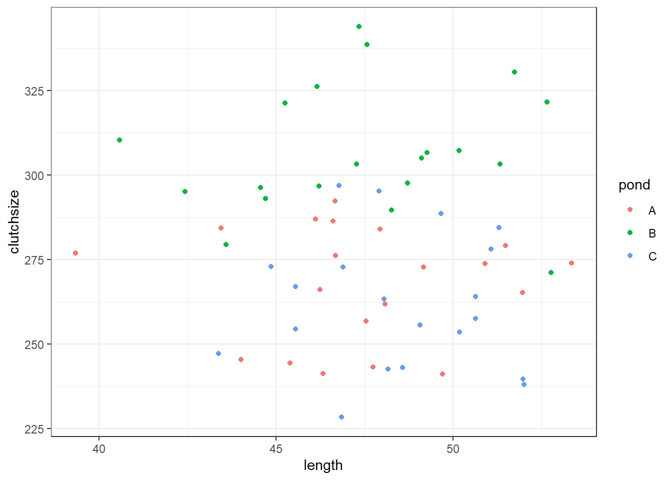
model = smf.ols(formula= "clutchsize ~ length + pond", data = goldentoad)

lm_golden = model.fit()
print(lm_golden.summary())
OLS Regression Results
==============================================================================
Dep. Variable: clutchsize R-squared: 0.354
Model: OLS Adj. R-squared: 0.319
Method: Least Squares F-statistic: 10.23
Date: Mon, 16 Mar 2026 Prob (F-statistic): 1.80e-05
Time: 17:26:16 Log-Likelihood: -263.47
No. Observations: 60 AIC: 534.9
Df Residuals: 56 BIC: 543.3
Df Model: 3
Covariance Type: nonrobust
==============================================================================
coef std err t P>|t| [0.025 0.975]
------------------------------------------------------------------------------
Intercept 196.9612 37.710 5.223 0.000 121.419 272.504
pond[T.B] 24.0615 6.419 3.749 0.000 11.204 36.919
pond[T.C] -10.4082 6.426 -1.620 0.111 -23.282 2.465
length 1.5491 0.781 1.984 0.052 -0.015 3.114
==============================================================================
Omnibus: 3.489 Durbin-Watson: 2.017
Prob(Omnibus): 0.175 Jarque-Bera (JB): 1.803
Skew: -0.074 Prob(JB): 0.406
Kurtosis: 2.164 Cond. No. 695.
==============================================================================
Notes:
[1] Standard Errors assume that the covariance matrix of the errors is correctly specified.Has our model recreated “reality” very well? Would we draw the right conclusions from it?
8.8 Exercises
8.8.1 A second categorical predictor
8.8.2 Continuing your own simulation
8.9 Summary
Whether our predictor is categorical or continuous, we still need to follow the same workflow to simulate the dataset.
However, categorical predictors are a touch more complicated to simulate - we need a couple of extra functions, and it’s conceptually a little harder to get used to.
TipKey Points
- Categorical predictors require vectors for their beta coefficients, unlike continuous predictors that just have constants
- This means we need to use a design matrix to multiply our vector beta coefficient by our categorical variable
- Otherwise, the procedure is identical to simulating with a continuous predictor
- You can include any number of continuous and categorical predictors in the same simulation