library(tidyverse)3 Drawing samples from distributions
3.1 Libraries and functions
NoteClick to expand
import pandas as pd
import numpy as np
import random
import statistics
import matplotlib.pyplot as plt
from plotnine import *
The first thing we need to get comfortable with is random sampling, i.e., drawing a number of data points from an underlying distribution with known parameters.
Parameters are features of a distribution that determine its shape. For example, the normal distribution has two parameters: mean and variance (or standard deviation).
This random sampling is what we’re (hopefully) doing when we collect a sample in experimental research. The underlying distribution of the response variable, i.e., the “ground truth” in the world, has some true parameters that we’re hoping to estimate. We collect a random subset of individual observations that have come from that underlying distribution, and use the sample’s statistics to estimate the true population parameters.
3.2 Sampling from the normal distribution
This is the rnorm function, which we’ll be using a lot in this course. It takes three arguments; the first is the number of data points (n) that you’d like to draw. The second and third arguments are the two important parameters that describe the shape of the underlying distribution: the mean and the standard deviation.
rnorm(n = 100, mean = 0, sd = 1) [1] -1.22940988 -0.78175473 -0.05941649 0.43406066 0.78549053 0.56536106
[7] -0.63515430 0.10417513 -2.08135144 -0.21772407 -0.36095027 1.25353619
[13] -1.31314589 0.96765067 -0.92081289 -0.76175924 0.73932670 1.10017197
[19] 0.12156430 -2.09315168 2.33844957 -0.22713777 -1.15659441 -0.50859259
[25] -0.35160684 -0.12091276 1.00008825 -0.90091916 -0.56267685 0.23064728
[31] -0.31785121 -0.58964684 -1.81563776 0.23640526 -1.20897085 1.12029491
[37] -0.38821684 1.13408684 -1.04606759 0.92615178 -0.09701480 -0.53382837
[43] -0.41569846 -0.25972174 -0.26645389 0.19264407 -0.91187099 0.42361118
[49] 1.42616047 -1.67701722 -1.14529965 -0.84394270 1.46987867 -0.01068597
[55] 0.49853952 2.47578333 0.05834657 0.33363704 -0.08329676 0.09074863
[61] 0.67496907 1.14087753 -1.04401976 0.14448116 -0.95568251 -0.06110808
[67] 0.04990981 -0.37881064 0.89040968 -0.50300805 0.90501630 -0.39382809
[73] 1.68724592 0.98484438 -0.41111495 -0.65825626 0.56220031 -1.06151990
[79] 0.80127211 -1.09972058 1.52686100 1.91600738 1.75376795 -0.46469303
[85] 0.28610037 1.19647158 -0.33322253 0.04652775 2.05441549 0.97647477
[91] -0.51554070 0.82428873 -0.62834756 -1.55123585 1.43185246 -0.16385640
[97] -0.15364102 2.47732635 0.45012856 0.92003779Without any further instruction, R simply prints us a list of length n; this list contains numbers that have been pulled randomly from a normal distribution with mean 0 and standard deviation 1.
This is a sample or dataset, drawn from an underlying population, which we can now visualise.
We’ll use the base R hist function for this for now, just to keep things simple:
rnorm(100, 0, 1) %>%
  hist()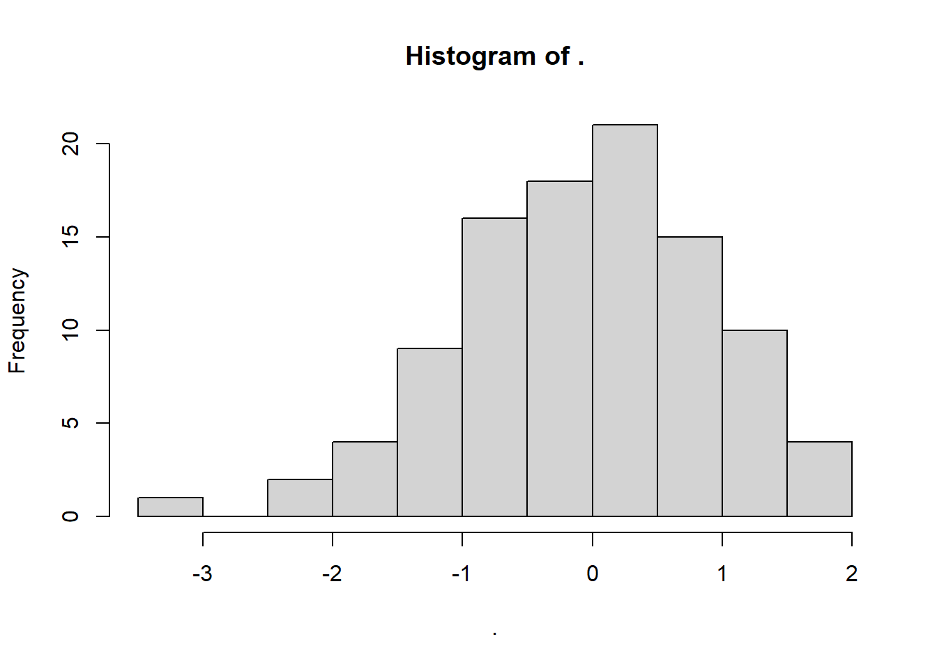
The typical default method in Python for sampling from a normal distribution is via numpy.random.normal.
It takes three arguments: loc (mean), scale (standard deviation) and size (sample size):
norm_data = np.random.normal(loc = 0, scale = 1, size = 100)
print(norm_data)
[ 1.18790953 1.38723105 -0.75600814 0.8410843 -0.57766845 -1.64258659
-0.50886713 1.5197107 0.86489165 0.3051659 0.68563204 -1.46101353
-0.74638774 0.31405489 0.10245238 0.88659415 -0.92750301 -0.16047263
0.96703509 -0.12210535 -1.21487207 0.35922202 0.49859833 -0.99115405
0.57701065 0.47599325 0.56958299 0.30291505 0.0988164 0.63402371
1.68415555 0.80163562 0.57098047 -1.04267593 0.76374138 -0.64495585
1.71271037 -1.10353423 -0.15160839 -0.2881727 0.40208074 0.18689907
2.50543842 0.84248958 0.11523662 0.13546877 0.63422016 -0.05847853
0.25498864 -0.61147325 -1.57169603 -1.29311285 0.42553885 0.93507036
-1.12242325 -0.11015332 0.88560299 -0.01718516 0.42783246 1.6490974
-1.01240318 -0.09587259 -0.26182404 -0.48902448 -1.23146388 1.37848657
-0.45180123 0.28357726 -0.47183027 -0.49051111 -2.5622498 -1.56173666
0.28948143 0.55626578 -0.57596352 -1.98400261 0.08957272 -1.10548904
0.27674145 0.00781173 1.81832078 1.10086291 -0.57059829 -0.2551952
1.00554561 2.11844184 -1.5444488 -0.79271778 -0.34570661 -0.32839502
1.25159258 -1.0947154 0.85876553 0.39134558 -0.79129755 0.46582172
-2.03891307 0.67608781 -2.73679991 1.21440739]The output is an array of numbers, of length size.
This is a sample or dataset, drawn from an underlying population, which we can now visualise.
For this first example, we’ll show how to use both matplotlib and plotnine to create histograms. We’ll use the matplotlib version for speed as we go through the course, but if you’re transitioning over from R (or ggplot), you might find plotnine friendlier.
plt.hist(norm_data)
plt.show()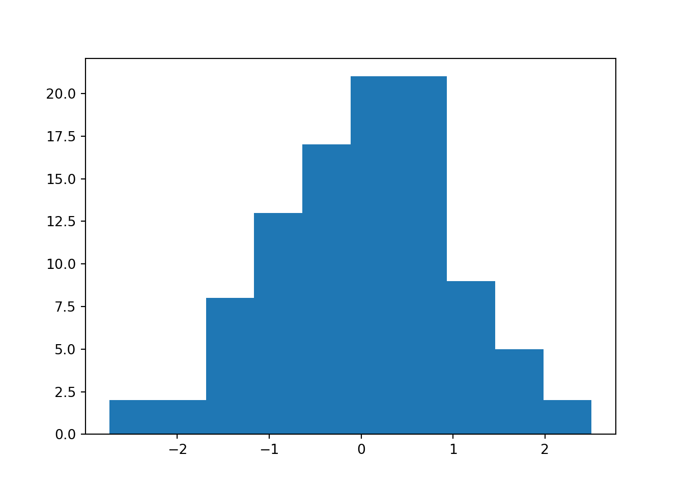
If plotting multiple histograms, you can use plt.clf() to clear the figure, or plt.close() to close the plotting window entirely.
If using plotnine, you have to convert the array to a data frame before you can visualise it:
norm_df = pd.DataFrame({"values":norm_data})

norm_df_hist = (
  ggplot(norm_df, aes(x = "values")) +
  geom_histogram()
)

print(norm_df_hist)
<ggplot: (640 x 480)>3.3 Sampling from other distributions
The normal/Gaussian distribution might be the most famous of the distributions, but it is not the only one that exists - nor the only one that we’ll care about on this course.
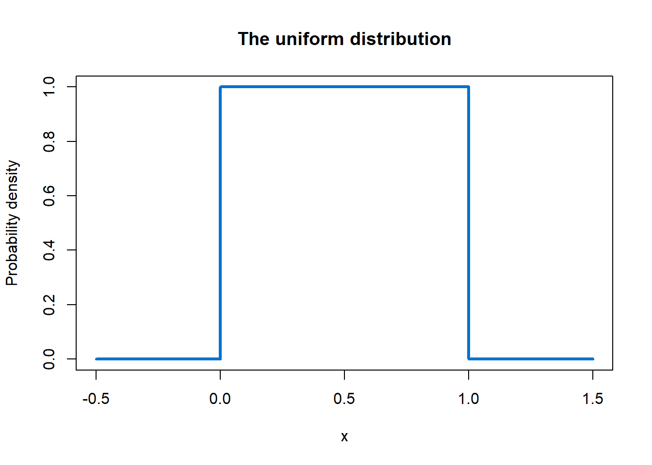
For example, we’ll also be sampling quite regularly from the uniform distribution.
The uniform distribution is flat: inside the range of possible values, all values are equally likely, and outside that range, the probability density drops to zero. This means the only parameters we need to set are the minimum and maximum of that range of possible values, like so:
runif(n = 100, min = 0, max = 1) %>%
  hist(xlim = c(-0.5, 1.5))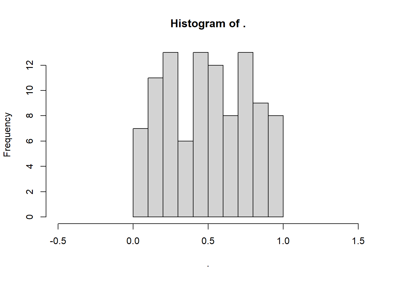
unif_data = np.random.uniform(low = 0, high = 1, size = 100)

plt.clf() # clear existing plot, if applicable
plt.hist(unif_data)
plt.show()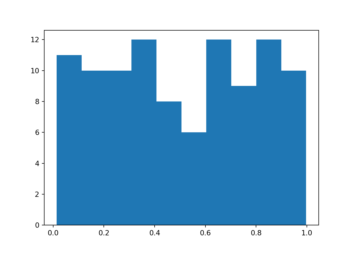
The underlying shape of the distribution that we just sampled from looks like this - square and boxy. The probability density is zero outside of the 0-1 range, and flat inside it:
Later in this course, we will sample from the binomial, negative binomial and Poisson distributions as well.
3.4 Setting a seed
What happens if you run this block of code over and over again?
rnorm(100, 0, 1) %>%
  hist()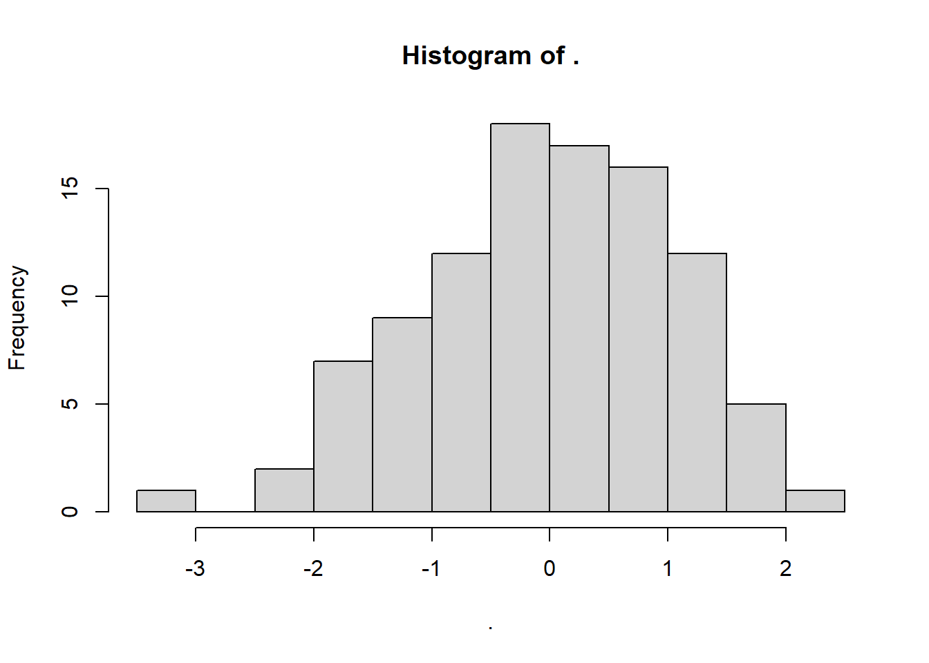
plt.clf()
plt.hist(np.random.normal(0, 1, 100))
plt.show()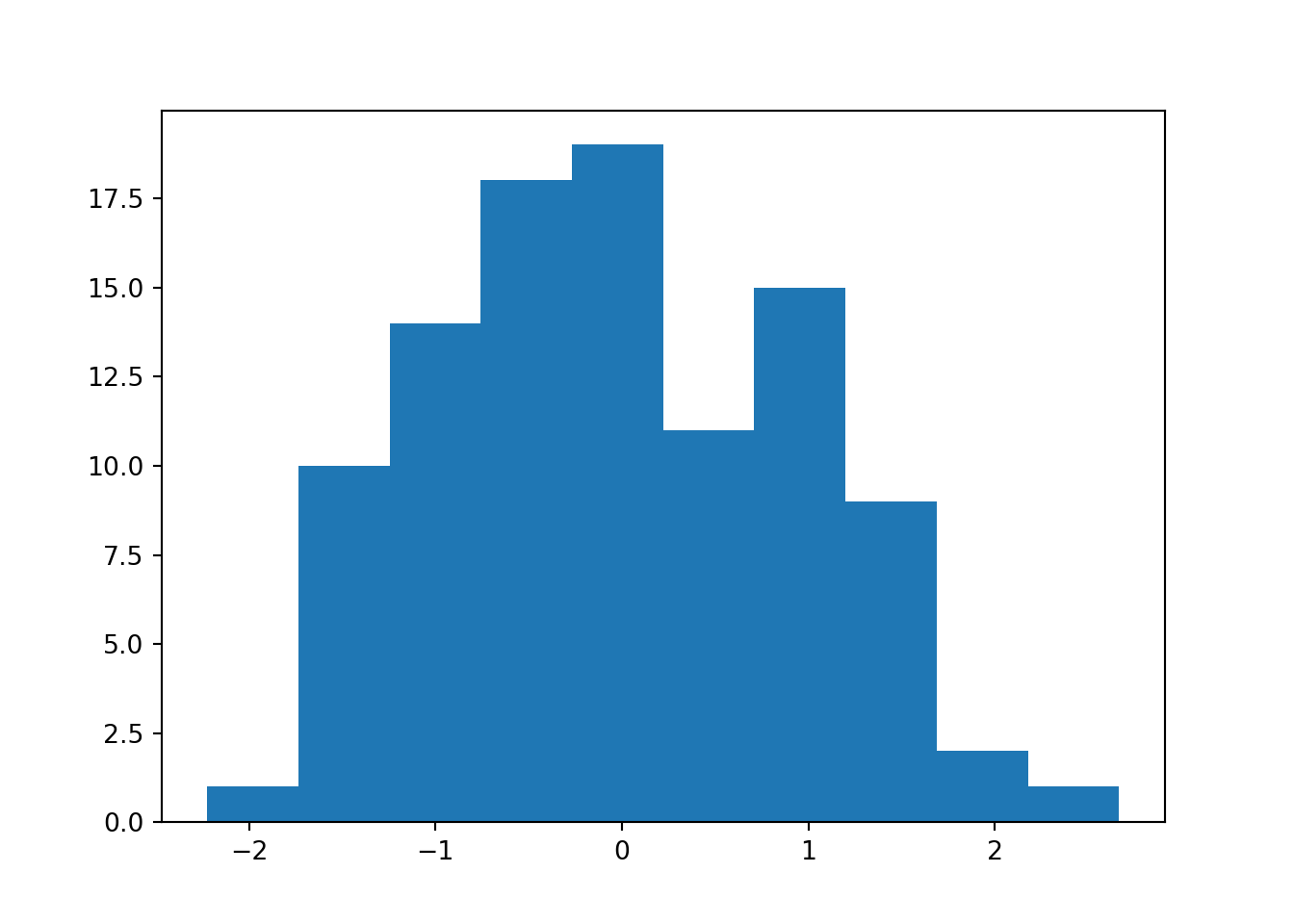
Each time you run the code, you are sampling a unique random subset of data points.
It’s very helpful that we can do that - later on in this course, we’ll exploit this to sample many different datasets from the same underlying population.
However, sometimes it’s useful for us to be able to sample the exact set of data points more than once.
To achieve this, we can use the set.seed function.
Run the following code several times in a row, and you’ll see the difference:
set.seed(20)

rnorm(100, 0, 1) %>%
  hist()
To achieve this, we can use the np.random.seed function.
Run the following code several times in a row, and you’ll see the difference:
np.random.seed(20)

plt.clf()
plt.hist(np.random.normal(0, 1, 100))
plt.show()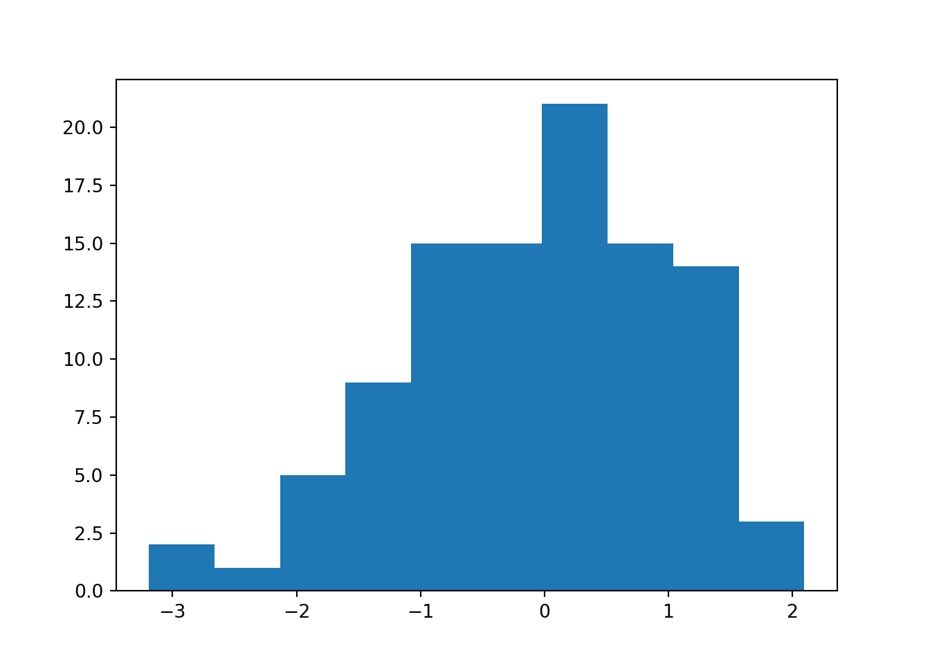
Notice how each time, the exact same dataset and histogram are produced?
You can choose any number you like for the seed. All that matters is that you return to that same seed number, if you want to recreate that dataset.
3.5 Exercises
3.5.1 Revisiting Shapiro-Wilk
Now that you know how to perform random sampling, let’s link it back to a specific statistical test, the Shapiro-Wilk test.
As a reminder: the Shapiro-Wilk test is used to help us decide whether a sample has been drawn from a normal distribution or not. It’s one of the methods we have for checking the normality assumption.
However, it is also itself a null hypothesis test. The null hypothesis is that the underlying distribution is normal, so a significant p-value is usually interpreted as evidence that the normality assumption is violated.
ExerciseExercise 1
Level:
In this exercise, using the template code provided as a starting point:
- Try a variety of different seeds (hint:
20might be interesting…) - Sample from a uniform distribution instead
- While sampling from both normal and uniform distributions, try a variety of sample sizes (including
n < 10) - Create normal QQ plots, to compare them to the Shapiro-Wilk results (use the
qqnormfunction)
Try to create:
- A false positive error
- A false negative error
What does this teach you about the nature of the Shapiro-Wilk test, and null hypothesis significance tests in general?
Template code:
set.seed(200)
n <- 100
Mean <- 0
SD <- 1

data <- rnorm(n, Mean, SD)

data %>% hist()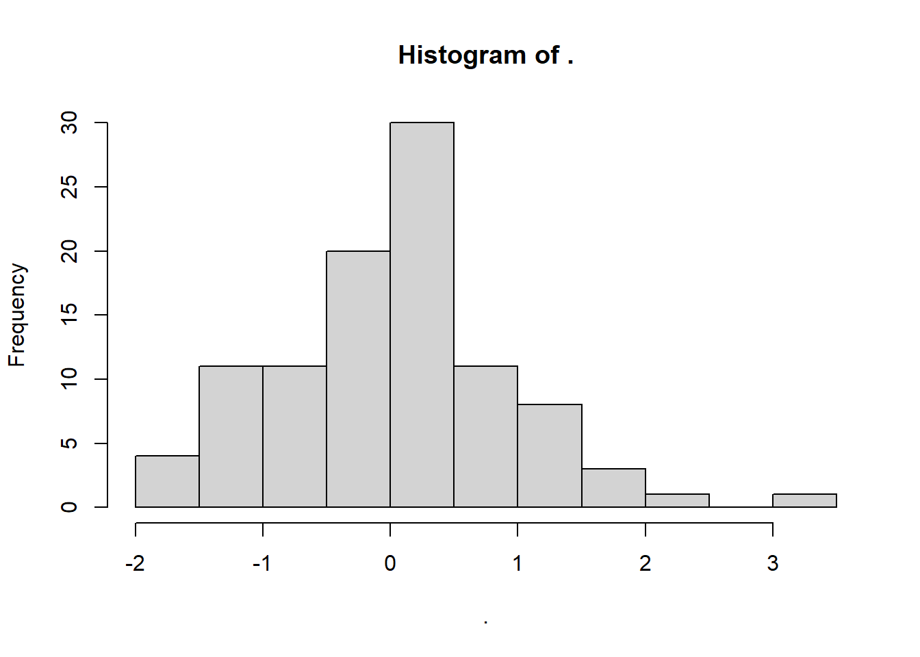
data %>% shapiro.test()
    Shapiro-Wilk normality test

data:  .
W = 0.97978, p-value = 0.1279
Template code:
import pingouin as pg # needed for the pg.normality function

np.random.seed(200)
n = 100
mean = 0
sd = 1

data = np.random.normal(mean, sd, n)

plt.clf()
plt.hist(data)
plt.show()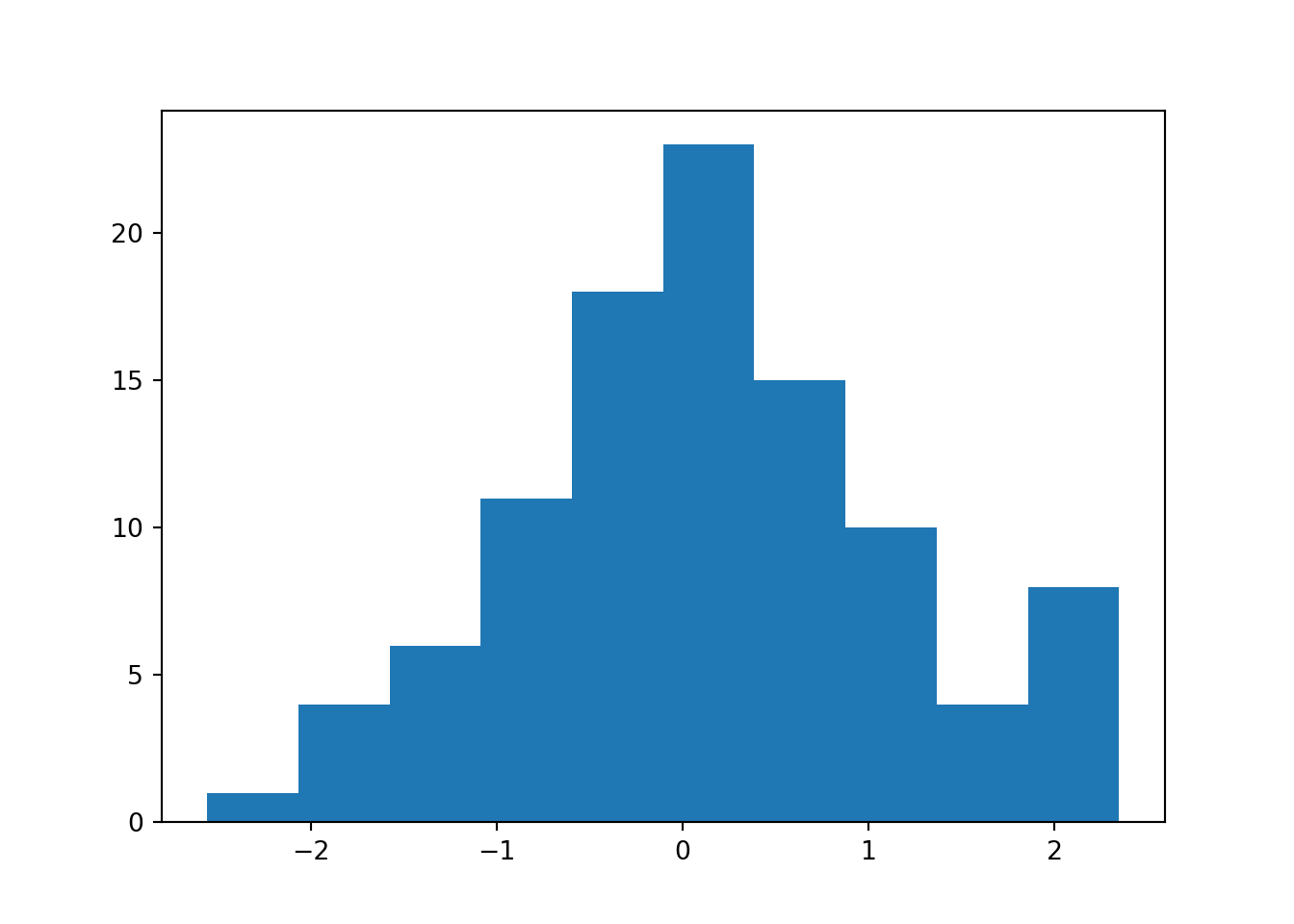
pg.normality(data) W pval normal
0 0.986137 0.382255 True3.6 Summary
This chapter introduced a key simulation concept: sampling from distributions with known parameters. This is central to all of the simulating we will do in the remaining chapters.
TipKey Points
- There are a suite of functions for sampling data points from distributions with known parameters
- Each distribution has its own function, with different parameters that we need to specify
- You can set a seed to make sure you sample the exact same set of values each time