15  Live demo exercises

15.1 Section setup

R

library(tidyverse)

Python

# A Python data analysis and manipulation tool
import pandas as pd

# Python equivalent of `ggplot2`
from plotnine import *

# If using seaborn for plotting
import seaborn as sns
import matplotlib.pyplot as plt

15.2 DA1: getting started

This is a hands-on demo.

R

Live demo RStudio:

• open RStudio
• highlight panels
• change default settings (.Rdata and not save workspace)
• set up new RProject data-analysis
• create the subfolders (data, images, scripts)
• create a script
• download and copy the data files into data

Python

Live demo JupyterLab:

• open JupyterLab
• highlight Launcher
• show how to check working directory, change if needed (data-analysis)
• create the subfolders (data, images, scripts)
• create a Notebook
• download and copy the data files into data

15.3 DA1: data types

Important to realise that there often is some order to how data types are interpreted. For example, look at the following:

R

example <- c(22, 87, NA, 32)

class(example)

[1] "numeric"

example <- c(22, 87, NA, "unsure")

class(example)

[1] "character"

Python

15.4 DA1: indexing

A bit of a technical detail, but an important one, particularly if you’re using both R and Python. The main focus of the example is not on the subsetting, it’s on the fact that R has 1-based indexing and Python has 0-based indexing.

Furthermore, that R’s indexing is inclusive, and Python’s exclusive (comparing 1:3 in R vs Python). That said, it’s to create awareness of the fact that indexing has to start somewhere and that it can be different between programming languages.

R

winnings <- c("first", "second", "third", "fourth")

The positional index is as follows:

seq_along(winnings)

[1] 1 2 3 4

So, if we wanted to select the first and third values, we’d do:

winnings[c(1, 3)]

[1] "first" "third"

Python

winnings = ["first", "second", "third", "fourth"]

The positional index is as follows:

list(range(len(winnings)))

[0, 1, 2, 3]

So, if we wanted to select the first and third values, we’d do:

winnings[0]

'first'

winnings[2]

'third'

15.5 DA2: data exploration

R

Read in the data:

infections <- read_csv("data/infections.csv")

And have a look:

head(infections)

# A tibble: 6 × 11
  patient_id hospital   quarter infection_type vaccination_status age_group
  <chr>      <chr>      <chr>   <chr>          <chr>              <chr>    
1 ID_0001    hospital_3 Q2      none           <NA>               65+      
2 ID_0002    hospital_3 Q2      viral          <NA>               18 - 64  
3 ID_0003    hospital_2 Q2      none           unknown            65+      
4 ID_0004    hospital_2 Q3      fungal         unvaccinated       < 18     
5 ID_0005    hospital_3 Q2      fungal         vaccinated         65+      
6 ID_0006    hospital_5 Q3      none           vaccinated         65+      
# ℹ 5 more variables: icu_admission <lgl>, symptoms_count <dbl>,
#   systolic_pressure <dbl>, body_temperature <dbl>, crp_level <dbl>

Python

Read in the data:

infections = pd.read_csv("data/infections.csv")

And have a look:

infections.head()

  patient_id    hospital  ... body_temperature crp_level
0    ID_0001  hospital_3  ...             37.8     12.05
1    ID_0002  hospital_3  ...             39.1      8.11
2    ID_0003  hospital_2  ...             38.5      5.24
3    ID_0004  hospital_2  ...             39.4     41.73
4    ID_0005  hospital_3  ...             36.9     10.51

[5 rows x 11 columns]

15.5.1 Data structure

Number of rows & columns:

R

nrow(infections)

[1] 1400

ncol(infections)

[1] 11

Python

infections.shape[0]

1400

infections.shape[1]

11

It’s good to look at the column attributes: what type of columns are we dealing with and is it what we expect?

R

summary(infections)

  patient_id          hospital           quarter          infection_type    
 Length:1400        Length:1400        Length:1400        Length:1400       
 Class :character   Class :character   Class :character   Class :character  
 Mode  :character   Mode  :character   Mode  :character   Mode  :character  
                                                                            
                                                                            
                                                                            
                                                                            
 vaccination_status  age_group         icu_admission   symptoms_count  
 Length:1400        Length:1400        Mode :logical   Min.   : 0.000  
 Class :character   Class :character   FALSE:814       1st Qu.: 6.000  
 Mode  :character   Mode  :character   TRUE :513       Median : 9.000  
                                       NA's :73        Mean   : 8.549  
                                                       3rd Qu.:11.000  
                                                       Max.   :21.000  
                                                       NA's   :67      
 systolic_pressure body_temperature   crp_level     
 Min.   : 87.0     Min.   :36.30    Min.   : 1.000  
 1st Qu.:118.0     1st Qu.:38.20    1st Qu.: 9.117  
 Median :125.0     Median :38.80    Median :16.215  
 Mean   :125.1     Mean   :38.75    Mean   :19.465  
 3rd Qu.:132.0     3rd Qu.:39.40    3rd Qu.:26.433  
 Max.   :163.0     Max.   :41.50    Max.   :58.860  
 NA's   :74        NA's   :67       NA's   :156     

str(infections)

spc_tbl_ [1,400 × 11] (S3: spec_tbl_df/tbl_df/tbl/data.frame)
 $ patient_id        : chr [1:1400] "ID_0001" "ID_0002" "ID_0003" "ID_0004" ...
 $ hospital          : chr [1:1400] "hospital_3" "hospital_3" "hospital_2" "hospital_2" ...
 $ quarter           : chr [1:1400] "Q2" "Q2" "Q2" "Q3" ...
 $ infection_type    : chr [1:1400] "none" "viral" "none" "fungal" ...
 $ vaccination_status: chr [1:1400] NA NA "unknown" "unvaccinated" ...
 $ age_group         : chr [1:1400] "65+" "18 - 64" "65+" "< 18" ...
 $ icu_admission     : logi [1:1400] FALSE FALSE TRUE TRUE TRUE FALSE ...
 $ symptoms_count    : num [1:1400] 1 6 3 7 7 5 10 12 13 7 ...
 $ systolic_pressure : num [1:1400] 117 115 120 129 114 124 133 120 124 127 ...
 $ body_temperature  : num [1:1400] 37.8 39.1 38.5 39.4 36.9 36.8 39.4 39.3 39.6 39.1 ...
 $ crp_level         : num [1:1400] 12.05 8.11 5.24 41.73 10.51 ...
 - attr(*, "spec")=
  .. cols(
  ..   patient_id = col_character(),
  ..   hospital = col_character(),
  ..   quarter = col_character(),
  ..   infection_type = col_character(),
  ..   vaccination_status = col_character(),
  ..   age_group = col_character(),
  ..   icu_admission = col_logical(),
  ..   symptoms_count = col_double(),
  ..   systolic_pressure = col_double(),
  ..   body_temperature = col_double(),
  ..   crp_level = col_double()
  .. )
 - attr(*, "problems")=<externalptr> 

Python

infections.describe()

       symptoms_count  systolic_pressure  body_temperature    crp_level
count     1333.000000        1326.000000       1333.000000  1244.000000
mean         8.549137         125.070136         38.751988    19.464751
std          3.825004          10.346761          0.883689    13.083907
min          0.000000          87.000000         36.300000     1.000000
25%          6.000000         118.000000         38.200000     9.117500
50%          9.000000         125.000000         38.800000    16.215000
75%         11.000000         132.000000         39.400000    26.432500
max         21.000000         163.000000         41.500000    58.860000

15.5.2 Quality control checks

It’s good to do some basic sanity / quality control checks. For example, if there are different categories in a column, do all the categories we expect show up or are there missing ones / misspelled etc.?

For example, we can check the unique values in a column:

R

unique(infections$infection_type)

[1] "none"      "viral"     "fungal"    NA          "bacterial"

Python

infections["infection_type"].unique()

array(['none', 'viral', 'fungal', nan, 'bacterial'], dtype=object)

We can count the number of missing values in the column infection_type.

R

You read the code “inside-out”:

sum(is.na(infections$infection_type))

[1] 74

Python

infections["infection_type"].isna().sum()

74

15.6 DA2: subsetting tables

Let’s select patient_id:

R

infections$patient_id

Python

infections.patient_id

0       ID_0001
1       ID_0002
2       ID_0003
3       ID_0004
4       ID_0005
         ...   
1395    ID_1396
1396    ID_1397
1397    ID_1398
1398    ID_1399
1399    ID_1400
Name: patient_id, Length: 1400, dtype: object

Or more than 1 column, by column name:

R

infections[, c("patient_id", "systolic_pressure")]

# A tibble: 1,400 × 2
   patient_id systolic_pressure
   <chr>                  <dbl>
 1 ID_0001                  117
 2 ID_0002                  115
 3 ID_0003                  120
 4 ID_0004                  129
 5 ID_0005                  114
 6 ID_0006                  124
 7 ID_0007                  133
 8 ID_0008                  120
 9 ID_0009                  124
10 ID_0010                  127
# ℹ 1,390 more rows

Python

infections[["patient_id", "systolic_pressure"]]

     patient_id  systolic_pressure
0       ID_0001              117.0
1       ID_0002              115.0
2       ID_0003              120.0
3       ID_0004              129.0
4       ID_0005              114.0
...         ...                ...
1395    ID_1396              118.0
1396    ID_1397              117.0
1397    ID_1398              137.0
1398    ID_1399              135.0
1399    ID_1400              129.0

[1400 rows x 2 columns]

Combine this with selecting only a subset of rows, let’s say the first three rows.

R

infections[1:3, c("patient_id", "systolic_pressure")]

# A tibble: 3 × 2
  patient_id systolic_pressure
  <chr>                  <dbl>
1 ID_0001                  117
2 ID_0002                  115
3 ID_0003                  120

Python

We need to be aware of the zero-based indexing, also noting that the value after the : is not included:

infections[["patient_id", "systolic_pressure"]].iloc[0:3]

  patient_id  systolic_pressure
0    ID_0001              117.0
1    ID_0002              115.0
2    ID_0003              120.0

15.7 DA2: simple plots

Let’s start with a simple scatterplot, where we plot body_temperature on the x-axis and crp_level on the y-axis.

R

ggplot(infections, aes(x = body_temperature, y = crp_level)) +
  geom_point()

Warning: Removed 215 rows containing missing values or values outside the scale range
(`geom_point()`).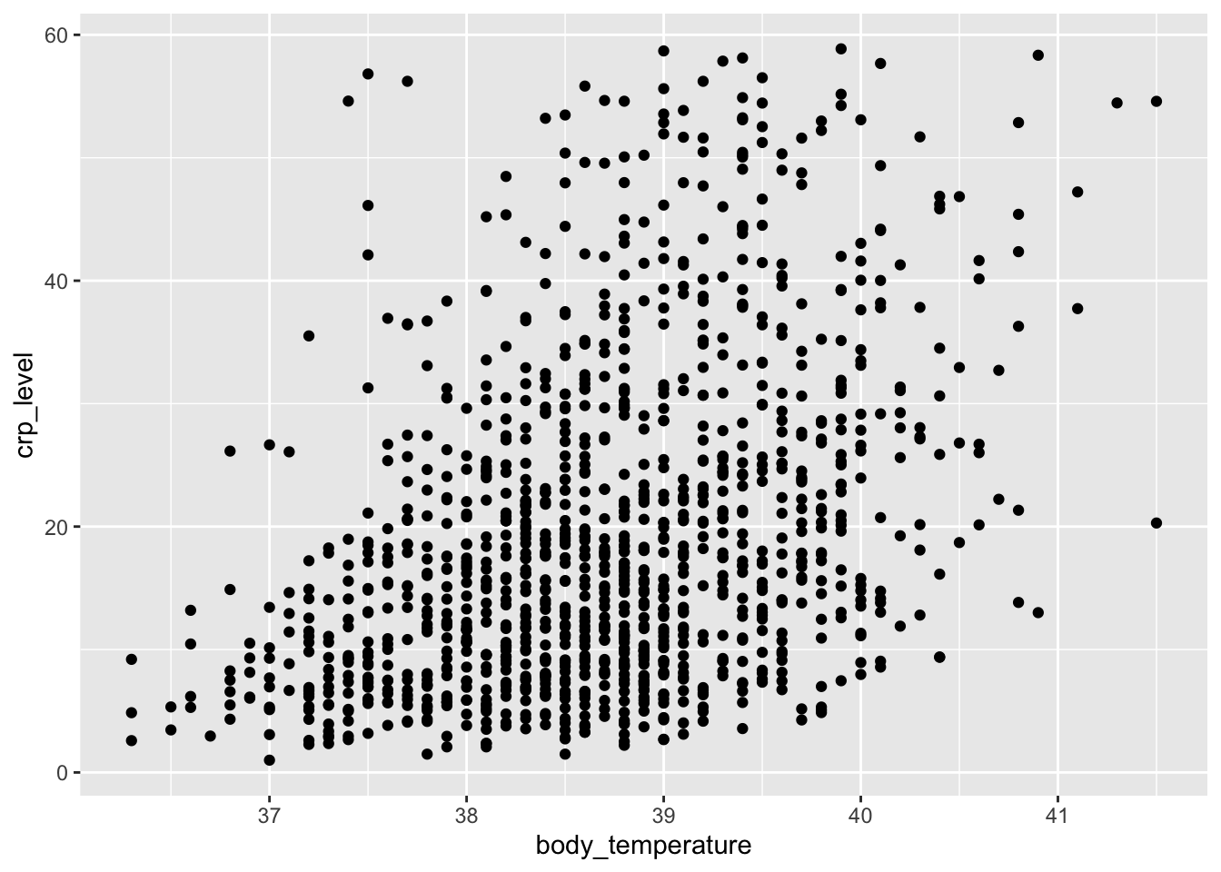

Python

p = (ggplot(infections, aes(x = "body_temperature", y = "crp_level")) +
  geom_point())
  
p.show()

We can explore this a bit further. For example, we can colour the points based on the hospital variable, to see if there are any patterns across the different hospitals:

R

ggplot(infections, aes(x = body_temperature, y = crp_level,
                       colour = hospital)) +
  geom_point()

Warning: Removed 215 rows containing missing values or values outside the scale range
(`geom_point()`).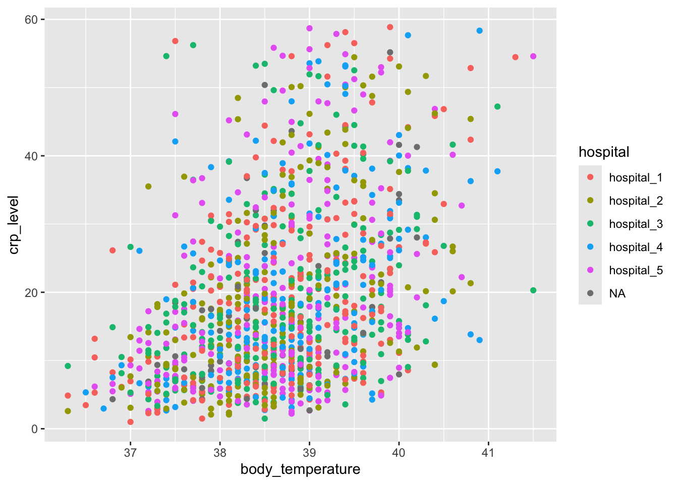

Python

p = (ggplot(infections, aes(x = "body_temperature", y = "crp_level",
                            colour = "hospital")) +
  geom_point())
  
p.show()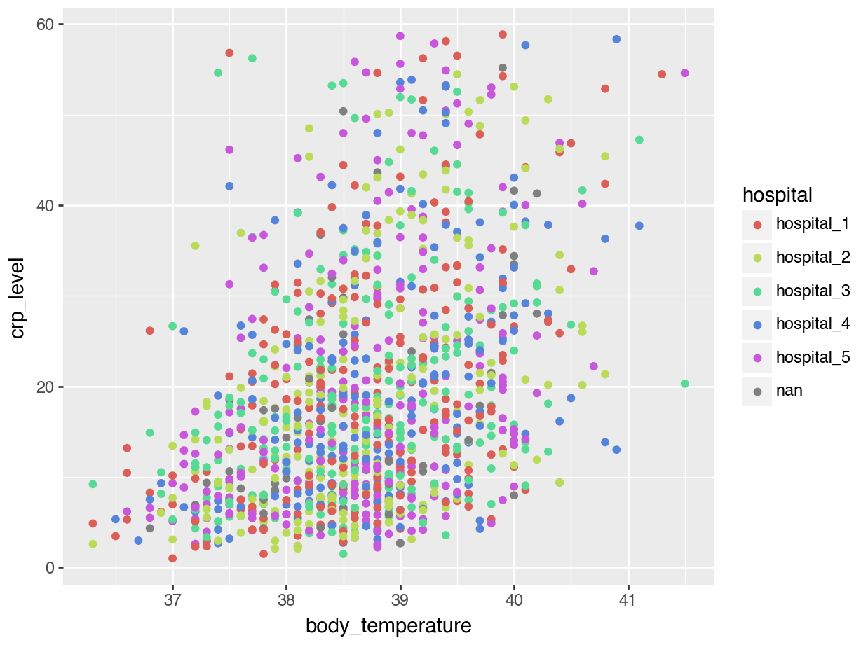

15.8 DA2: facetting data

When we plotted body_temperature and crp_level against each other and coloured the data based on hospital, we ended up with a rather unclear plot. This is probably because there are no clear differences between the hospitals. However, we can separate these data a bit more clearly by using facets.

R

ggplot(infections, aes(x = body_temperature, y = crp_level,
                       colour = hospital)) +
  geom_point() +
  facet_wrap(facets = vars(hospital))

Warning: Removed 215 rows containing missing values or values outside the scale range
(`geom_point()`).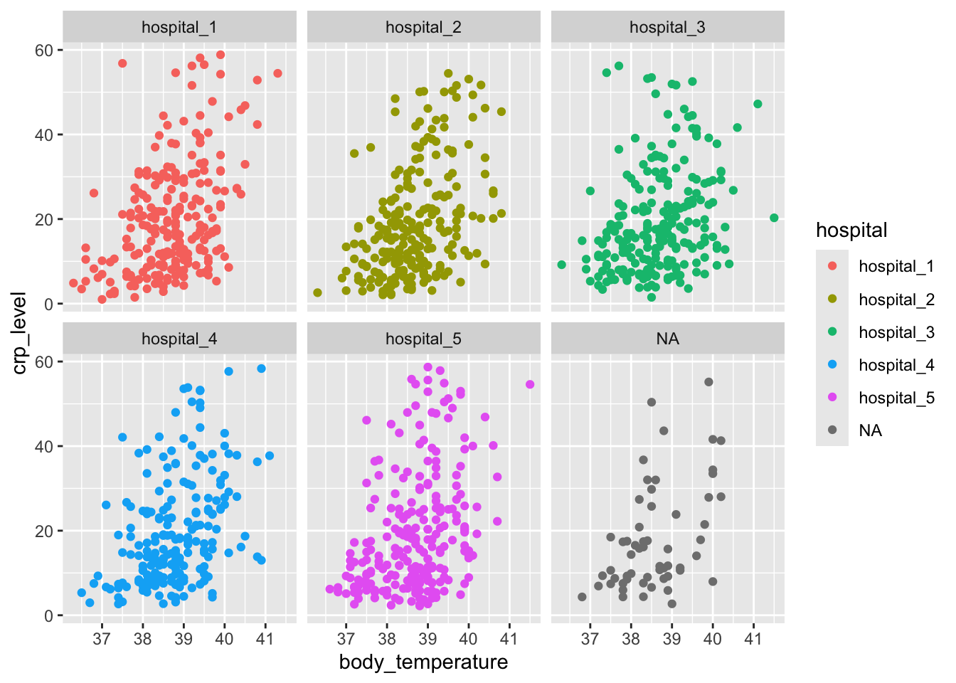

  ggplot(infections, aes(x = body_temperature, y = crp_level,
                         colour = hospital)) +
    geom_point() +
    facet_grid(rows = vars(icu_admission), cols = vars(hospital))

Warning: Removed 215 rows containing missing values or values outside the scale range
(`geom_point()`).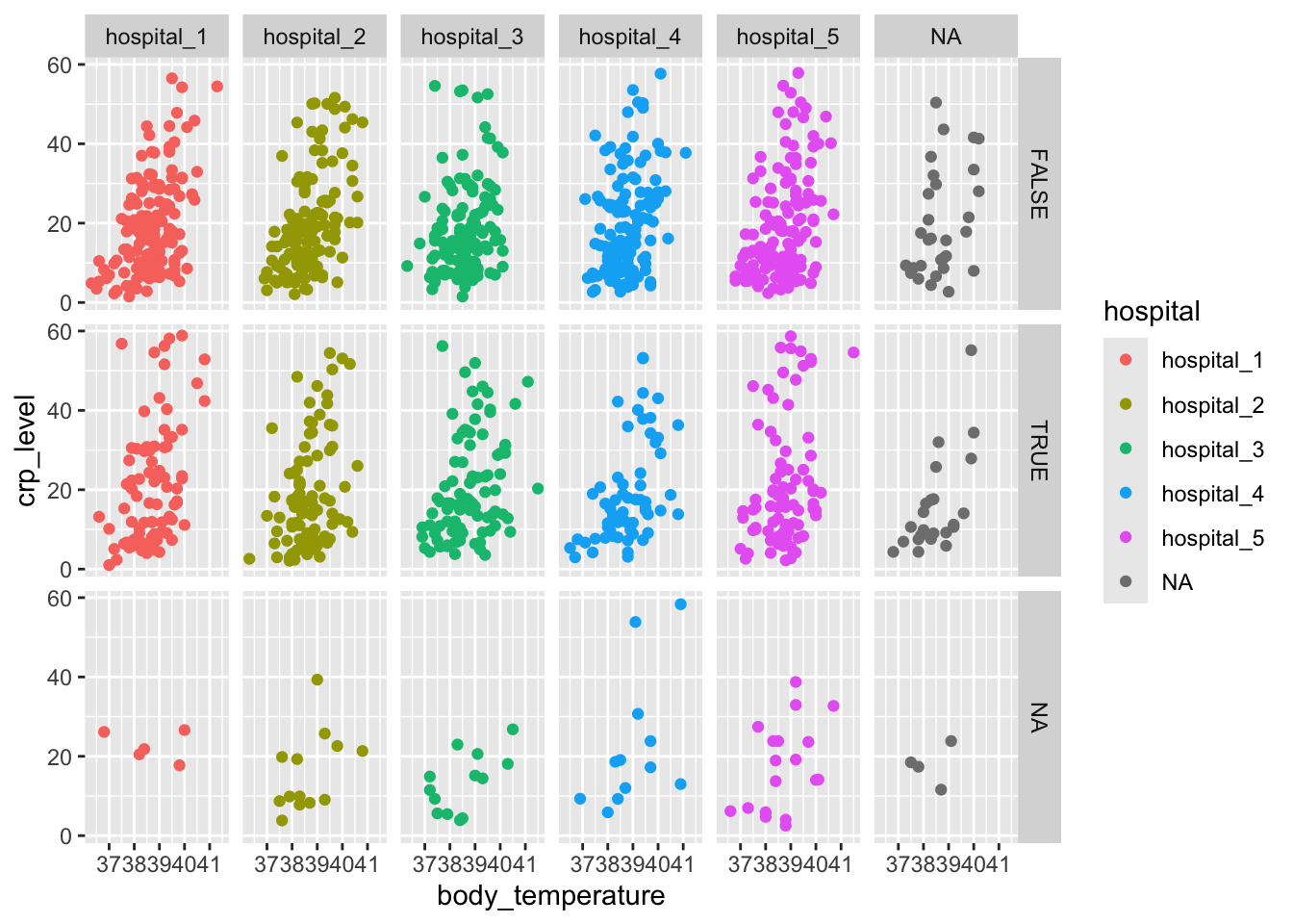

Python

p = (ggplot(infections, aes(x = "body_temperature", y = "crp_level",
                            colour = "hospital")) +
  geom_point() +
  facet_wrap("~ hospital"))
  
p.show()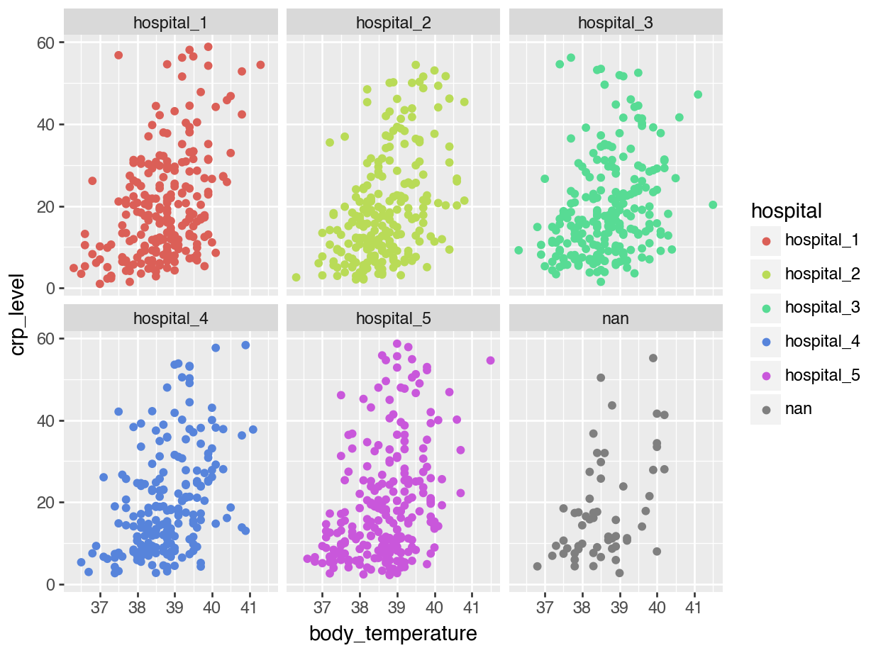

15.9 DA3: selecting columns

We’re practising two things:

1. selecting columns
2. creating columns (and highlight the use by plotting)

Let’s see which columns we have:

R

colnames(infections)

 [1] "patient_id"         "hospital"           "quarter"           
 [4] "infection_type"     "vaccination_status" "age_group"         
 [7] "icu_admission"      "symptoms_count"     "systolic_pressure" 
[10] "body_temperature"   "crp_level"         

Python

Let’s say we only wanted to select some of these.

R

select(infections, patient_id, body_temperature)

# A tibble: 1,400 × 2
   patient_id body_temperature
   <chr>                 <dbl>
 1 ID_0001                37.8
 2 ID_0002                39.1
 3 ID_0003                38.5
 4 ID_0004                39.4
 5 ID_0005                36.9
 6 ID_0006                36.8
 7 ID_0007                39.4
 8 ID_0008                39.3
 9 ID_0009                39.6
10 ID_0010                39.1
# ℹ 1,390 more rows

Python

Or select by data type:

R

select(infections, where(is.numeric))

# A tibble: 1,400 × 4
   symptoms_count systolic_pressure body_temperature crp_level
            <dbl>             <dbl>            <dbl>     <dbl>
 1              1               117             37.8     12.0 
 2              6               115             39.1      8.11
 3              3               120             38.5      5.24
 4              7               129             39.4     41.7 
 5              7               114             36.9     10.5 
 6              5               124             36.8      6.57
 7             10               133             39.4     53.1 
 8             12               120             39.3     NA   
 9             13               124             39.6     50.3 
10              7               127             39.1     13.0 
# ℹ 1,390 more rows

Python

Or based on a certain phrase within the column heading:

R

select(infections, contains("_id"))

# A tibble: 1,400 × 1
   patient_id
   <chr>     
 1 ID_0001   
 2 ID_0002   
 3 ID_0003   
 4 ID_0004   
 5 ID_0005   
 6 ID_0006   
 7 ID_0007   
 8 ID_0008   
 9 ID_0009   
10 ID_0010   
# ℹ 1,390 more rows

Python

15.10 DA3: creating columns

There aren’t too many variables in our data set that we can transform. However, the CRP levels are a good example. The CRP (C-reactive protein) is a continuous biomarker, often used clinically to indicate inflammation or infection severity. It can be skewed at times, so scaling it could be useful if you’re making comparisons across groups.

NoteScaling vs log-transforming

This falls well outside the scope of this course, but it’s possible that the question comes up. We could also log-transform our data if there is an issue with skewing etc. Very simply & briefly put:

• use log() when the distribution shape is the issue (e.g. skew, tails)
• use scale() when the unit or range is the issue (often when comparing across different variables with different units)
• using both can also be helpful, where you log-transform first, then scale the data to use in modelling.

We can scale the data where, for each value, we subtract the mean and divide by the standard deviation.

R

In R, we can use the scale() function to do this.

mutate(infections, crp_scaled = scale(crp_level))

# A tibble: 1,400 × 12
   patient_id hospital   quarter infection_type vaccination_status age_group
   <chr>      <chr>      <chr>   <chr>          <chr>              <chr>    
 1 ID_0001    hospital_3 Q2      none           <NA>               65+      
 2 ID_0002    hospital_3 Q2      viral          <NA>               18 - 64  
 3 ID_0003    hospital_2 Q2      none           unknown            65+      
 4 ID_0004    hospital_2 Q3      fungal         unvaccinated       < 18     
 5 ID_0005    hospital_3 Q2      fungal         vaccinated         65+      
 6 ID_0006    hospital_5 Q3      none           vaccinated         65+      
 7 ID_0007    hospital_4 Q1      fungal         unvaccinated       18 - 64  
 8 ID_0008    hospital_1 Q1      <NA>           unvaccinated       18 - 64  
 9 ID_0009    hospital_2 Q1      viral          <NA>               65+      
10 ID_0010    hospital_3 Q3      none           unvaccinated       <NA>     
# ℹ 1,390 more rows
# ℹ 6 more variables: icu_admission <lgl>, symptoms_count <dbl>,
#   systolic_pressure <dbl>, body_temperature <dbl>, crp_level <dbl>,
#   crp_scaled <dbl[,1]>

Let’s store this in a temporary object, so we can visualise it.

example <- mutate(infections, crp_scaled = scale(crp_level))

We can then plot it, adding a reference line at y = 0.

ggplot(example, aes(x = quarter, y = crp_scaled)) +
  geom_jitter(width = 0.1) +
  geom_hline(yintercept = 0, colour = "blue", linewidth = 1)

Warning: Removed 156 rows containing missing values or values outside the scale range
(`geom_point()`).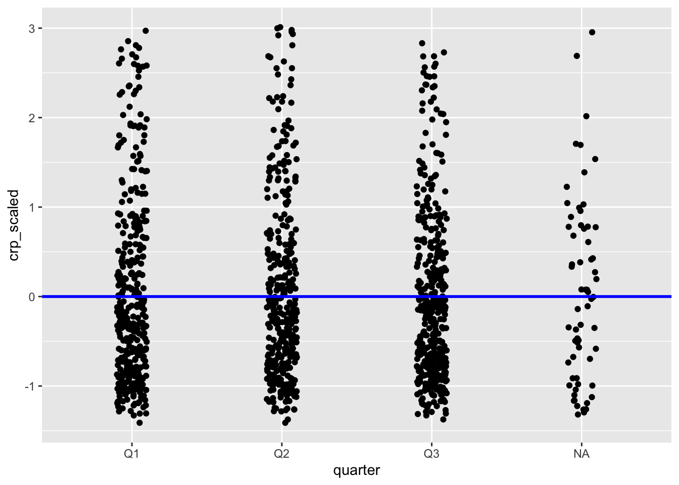

Python

15.11 DA3: creating columns (conditional)

Sometimes we need to create new columns based on certain conditions. Let’s say we wanted to flag if patients not vaccinated and have been admitted to ICU we consider them as high risk.

We want to encode this in a column risk_factor, where we label them as "high". This would then allow us to add other values, such as "low" or "medium" at a later time.

R

mutate(infections,
       risk_factor = ifelse(vaccination_status == "unvaccinated" & icu_admission == TRUE, "high", NA))

# A tibble: 1,400 × 12
   patient_id hospital   quarter infection_type vaccination_status age_group
   <chr>      <chr>      <chr>   <chr>          <chr>              <chr>    
 1 ID_0001    hospital_3 Q2      none           <NA>               65+      
 2 ID_0002    hospital_3 Q2      viral          <NA>               18 - 64  
 3 ID_0003    hospital_2 Q2      none           unknown            65+      
 4 ID_0004    hospital_2 Q3      fungal         unvaccinated       < 18     
 5 ID_0005    hospital_3 Q2      fungal         vaccinated         65+      
 6 ID_0006    hospital_5 Q3      none           vaccinated         65+      
 7 ID_0007    hospital_4 Q1      fungal         unvaccinated       18 - 64  
 8 ID_0008    hospital_1 Q1      <NA>           unvaccinated       18 - 64  
 9 ID_0009    hospital_2 Q1      viral          <NA>               65+      
10 ID_0010    hospital_3 Q3      none           unvaccinated       <NA>     
# ℹ 1,390 more rows
# ℹ 6 more variables: icu_admission <lgl>, symptoms_count <dbl>,
#   systolic_pressure <dbl>, body_temperature <dbl>, crp_level <dbl>,
#   risk_factor <chr>

Python

15.12 DA4: reshaping data

To illustrate reshaping data, we’re going to simplify our data set a little bit. First, we’ll calculate the average CRP levels for each hospital, quarter, infection type, vaccination status and age group.

We’ll use that summary table to highlight some use cases for reshaping data from a long to a wide format - and back.

15.12.1 Creating a summary table for CRP

R

infections_summary <- infections |> 
  drop_na() |> 
  group_by(hospital, quarter, infection_type, vaccination_status, age_group) |> 
  summarise(mean_crp = round(mean(crp_level, na.rm = TRUE), 2)) |> 
  ungroup()

`summarise()` has grouped output by 'hospital', 'quarter', 'infection_type',
'vaccination_status'. You can override using the `.groups` argument.

Let’s look at the output. We now have 6 columns, one for each of our grouping variables and at the end the mean_crp column containing the average CRP levels (rounded to two digits).

head(infections_summary)

# A tibble: 6 × 6
  hospital   quarter infection_type vaccination_status age_group mean_crp
  <chr>      <chr>   <chr>          <chr>              <chr>        <dbl>
1 hospital_1 Q1      bacterial      unknown            65+          23.7 
2 hospital_1 Q1      bacterial      unknown            < 18         25.8 
3 hospital_1 Q1      bacterial      unvaccinated       18 - 64       8.35
4 hospital_1 Q1      bacterial      unvaccinated       65+          23.2 
5 hospital_1 Q1      bacterial      unvaccinated       < 18         26.8 
6 hospital_1 Q1      bacterial      vaccinated         18 - 64      22.4 

Python

15.12.2 Wide table by quarter

Let’s say we’d be interested how the (average) CRP levels change over time across the different groupings. We’d be interested in having the mean_crp values for each quarter next to each other. That way we’d be able to plot quarterly average CRP levels against each other.

We can do this as follows:

R

infections_wide <- infections_summary |> 
  pivot_wider(names_from = "quarter",
              values_from = "mean_crp")

head(infections_wide)

# A tibble: 6 × 7
  hospital   infection_type vaccination_status age_group    Q1    Q2    Q3
  <chr>      <chr>          <chr>              <chr>     <dbl> <dbl> <dbl>
1 hospital_1 bacterial      unknown            65+       23.7   NA    26.8
2 hospital_1 bacterial      unknown            < 18      25.8   54.5  NA  
3 hospital_1 bacterial      unvaccinated       18 - 64    8.35  NA    NA  
4 hospital_1 bacterial      unvaccinated       65+       23.2   28.6  NA  
5 hospital_1 bacterial      unvaccinated       < 18      26.8   25.0  17.1
6 hospital_1 bacterial      vaccinated         18 - 64   22.4   12.7  NA  

Python

This then allows us to plot the data, for example:

R

ggplot(infections_wide, aes(x = Q1, y = Q2)) +
  geom_point() +
  geom_smooth(method = "lm", se = FALSE)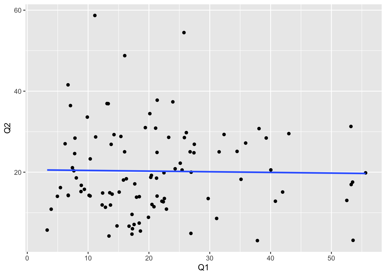

Python

15.12.3 Back to long format

We can revert back to a long format with the following:

R

pivot_longer(infections_wide,
             cols = Q1:Q3,           # columns to pivot
             names_to = "quarter",   # column for headings
             values_to = "mean_crp") # column for values

# A tibble: 534 × 6
   hospital   infection_type vaccination_status age_group quarter mean_crp
   <chr>      <chr>          <chr>              <chr>     <chr>      <dbl>
 1 hospital_1 bacterial      unknown            65+       Q1         23.7 
 2 hospital_1 bacterial      unknown            65+       Q2         NA   
 3 hospital_1 bacterial      unknown            65+       Q3         26.8 
 4 hospital_1 bacterial      unknown            < 18      Q1         25.8 
 5 hospital_1 bacterial      unknown            < 18      Q2         54.5 
 6 hospital_1 bacterial      unknown            < 18      Q3         NA   
 7 hospital_1 bacterial      unvaccinated       18 - 64   Q1          8.35
 8 hospital_1 bacterial      unvaccinated       18 - 64   Q2         NA   
 9 hospital_1 bacterial      unvaccinated       18 - 64   Q3         NA   
10 hospital_1 bacterial      unvaccinated       65+       Q1         23.2 
# ℹ 524 more rows

Python

And all is well with the world again.

15.13 DA4: joining data

In the infections data set we have a variable called hospital. This contains the following unique entries:

R

infections |> count(hospital)

# A tibble: 6 × 2
  hospital       n
  <chr>      <int>
1 hospital_1   277
2 hospital_2   259
3 hospital_3   280
4 hospital_4   245
5 hospital_5   271
6 <NA>          68

Python

Note that for some of the hospital entries there are missing data. This is relevant later on, when we’re joining.

We’re now going to add information on the hospitals, which are stored in hospital_info.csv. Let’s read in the data:

R

hospital_info <- read_csv("data/hospital_info.csv")

Python

Look at the data. There are 6 distinct hospital entries, with additional information for each hospital. We have the following variables:

Variable	Type	Description
hospital	character (id)	Unique hospital identifier (hospital_1 … hospital_6).
hospital_name	character	Official hospital name (e.g., Royal London Hospital).
location	character	City where the hospital is located (e.g., London, Manchester).
bed_capacity	integer	Approximate number of inpatient beds available at the hospital.
teaching_hospital	logical	Indicates if the hospital is a teaching hospital (TRUE / FALSE).

15.13.1 Left join

First, we’ll add the hospital_info data to the infections data set. We do this with a left-join. We expect hospital info data to be added to our main infections table, if the hospital value in infections matches with the one in hospital_info.

R

infections_left <- left_join(infections, hospital_info, by = "hospital")

Let’s just select the ID column from infections, together with all the columns that have been added.

infections_left |> 
  select(patient_id, hospital, hospital_name, location, bed_capacity, teaching_hospital) |> 
  head()

# A tibble: 6 × 6
  patient_id hospital   hospital_name    location bed_capacity teaching_hospital
  <chr>      <chr>      <chr>            <chr>           <dbl> <lgl>            
1 ID_0001    hospital_3 Bristol Royal I… Bristol           768 TRUE             
2 ID_0002    hospital_3 Bristol Royal I… Bristol           768 TRUE             
3 ID_0003    hospital_2 Manchester Gene… Manches…          849 FALSE            
4 ID_0004    hospital_2 Manchester Gene… Manches…          849 FALSE            
5 ID_0005    hospital_3 Bristol Royal I… Bristol           768 TRUE             
6 ID_0006    hospital_5 Cardiff Univers… Cardiff           582 TRUE             

We can see that the hospital information is now added to the data. We don’t expect any data to have dropped, so the number of observations/rows in infections_left should match the original 1400 from infections.

nrow(infections_left)

[1] 1400

Python

15.13.2 Right join

So, how does a right join then differ from a left join? Well, here we’d be adding the infections data to the hospital_info data (so, in the other direction). That means that for each hospital value that exists in hospital_info it will try and find the values that match the hospital column in infections.

R

infections_right <- right_join(infections, hospital_info, by = "hospital")

Again, the resulting table contains the data from both infections and hospital_info:

head(infections_right)

# A tibble: 6 × 15
  patient_id hospital   quarter infection_type vaccination_status age_group
  <chr>      <chr>      <chr>   <chr>          <chr>              <chr>    
1 ID_0001    hospital_3 Q2      none           <NA>               65+      
2 ID_0002    hospital_3 Q2      viral          <NA>               18 - 64  
3 ID_0003    hospital_2 Q2      none           unknown            65+      
4 ID_0004    hospital_2 Q3      fungal         unvaccinated       < 18     
5 ID_0005    hospital_3 Q2      fungal         vaccinated         65+      
6 ID_0006    hospital_5 Q3      none           vaccinated         65+      
# ℹ 9 more variables: icu_admission <lgl>, symptoms_count <dbl>,
#   systolic_pressure <dbl>, body_temperature <dbl>, crp_level <dbl>,
#   hospital_name <chr>, location <chr>, bed_capacity <dbl>,
#   teaching_hospital <lgl>

How many observations do we expect? Let’s have a look at how many we’ve got.

nrow(infections_right)

[1] 1333

Python

Here we see that we have fewer than the original 1400 observations, because we are joining in the other direction. Remember, there are missing values in our infections data set (68 in total). When we’re joining infections to hospital_info, these entries get dropped, because there is no missing value entry in the hospital column of hospital_info.

For the eagle-eyed amongst you: we have 1333 observations/rows in infections_right, whereas there are 68 missing values. We might have expected there to be 1332 rows (the difference between the number of rows in infections and the number of missing values), but there are 1333.

Why? Well, there is one entry in hospital_info that does not appear in infections: hospital_6. When we right join, this value gets retained, so this adds one additional row to the final output.

R

infections_right |> count(hospital)

# A tibble: 6 × 2
  hospital       n
  <chr>      <int>
1 hospital_1   277
2 hospital_2   259
3 hospital_3   280
4 hospital_4   245
5 hospital_5   271
6 hospital_6     1

Python

If we wouldn’t want that, we’d use inner join.

15.13.3 Inner join

Inner join will join two tables and only retain values (based on the joining ID) that exist in both tables.

R

infections_inner <- inner_join(infections, hospital_info, by = "hospital")

nrow(infections_inner)

[1] 1332

Only the 5 hospitals that appear in the infections data set are retained:

infections_inner |> count(hospital)

# A tibble: 5 × 2
  hospital       n
  <chr>      <int>
1 hospital_1   277
2 hospital_2   259
3 hospital_3   280
4 hospital_4   245
5 hospital_5   271

Python

This is entirely expected, since we don’t have missing data in hospital_info (so all the missing data from infections are dropped), nor do we have a hospital_6 entry in infections (so that is dropped too).

15.13.4 Full join

If we wanted to retain all observations, regardless of which table they’re from, we’d use a full join.

R

infections_full <- full_join(infections, hospital_info, by = "hospital")

How many rows do we expect? Well, the 1400 from infections plus the one extra (hospital_6 entry) from hospital_info:

nrow(infections_full)

[1] 1401

We can check that we’ve retained all values, by counting the number of observations for each hospital value:

infections_full |> count(hospital)

# A tibble: 7 × 2
  hospital       n
  <chr>      <int>
1 hospital_1   277
2 hospital_2   259
3 hospital_3   280
4 hospital_4   245
5 hospital_5   271
6 hospital_6     1
7 <NA>          68

Python

We see that all hospital values are retained, including the missing values and the one hospital_6 value coming from the hospital_info data set. Success!