# A collection of R packages designed for data science
library(tidyverse)

surveys <- read_csv("data/surveys.csv")
plot_types <- read_csv("data/plots.csv")
species <- read_csv("data/species.csv")13 Combining data
TipLearning objectives
- Learn how to join two tables together.
- Be able to distinguish between different types of joins.
- Use filtering joins to identify (mis)matches between tables.
13.1 Context
Data is often split over multiple tables. We saw this in the previous section. Sometimes we need to combine information from multiple sources.
13.2 Section setup
We’ll continue this section with the script named 04_session. If needed, add the following code to the top of your script and run it.
We’ll continue this section with the Notebook named 04_session. Add the following code to the first cell and run it.
# A Python data analysis and manipulation tool
import pandas as pd

# Python equivalent of `ggplot2`
from plotnine import *

# If using seaborn for plotting
import seaborn as sns
import matplotlib.pyplot as plt

surveys = pd.read_csv("data/surveys.csv")
plot_types = pd.read_csv("data/plots.csv")
species = pd.read_csv("data/species.csv")
13.3 Joining tables
We’ve already seen that some of our data sets have an identifier, for example the record_id in the surveys data set.
When it comes to joining data, these identifiers become extra important. After all, we need to be able to tell the computer how to join the data. We do this through a common key or variable between two data sets. We’ll illustrate how this works below.
13.3.1 Setting up your joins
There are different ways you can join tables, depending on which data you’d like to retain. The way these joins are named often depend on the direction in which you are joining. Let’s look at this in more detail, using examples.
plot_types <- read_csv("data/plots.csv")Rows: 5 Columns: 2
── Column specification ────────────────────────────────────────────────────────
Delimiter: ","
chr (1): plot_type
dbl (1): plot_id
ℹ Use `spec()` to retrieve the full column specification for this data.
ℹ Specify the column types or set `show_col_types = FALSE` to quiet this message.Let’s look at the data. We can see that there are five distinct plot types encoded in these data, using plot_id as a key.
plot_types# A tibble: 5 × 2
plot_id plot_type
<dbl> <chr>
1 1 Spectab exclosure
2 2 Control
3 3 Long-term Krat Exclosure
4 4 Rodent Exclosure
5 5 Short-term Krat ExclosureNow let’s look at our surveys data set. We know we have a plot_id column there, too. Let’s check how many times the different plot_id values occur in our data. For this, we can use the count() function:
surveys |> count(plot_id)# A tibble: 24 × 2
plot_id n
<dbl> <int>
1 1 1995
2 2 2194
3 3 1828
4 4 1969
5 5 1194
6 6 1582
7 7 816
8 8 1891
9 9 1936
10 10 469
# ℹ 14 more rowsThis shows that there are 24 plot_id values (there are 24 rows in the output). So, the plot_types data set won’t contain information on all of these, since it only contains 5 distinct plots.
plot_types = pd.read_csv("data/plots.csv")Let’s look at the data. We can see that there are five distinct plot types encoded in these data, using plot_id as a key.
plot_types plot_id plot_type
0 1 Spectab exclosure
1 2 Control
2 3 Long-term Krat Exclosure
3 4 Rodent Exclosure
4 5 Short-term Krat ExclosureNow let’s look at our surveys data set. We know we have a plot_id column there, too. Let’s check how many times the different plot_id values occur in our data.
surveys.groupby('plot_id').size().reset_index(name='n') plot_id n
0 1 1995
1 2 2194
2 3 1828
3 4 1969
4 5 1194
5 6 1582
6 7 816
7 8 1891
8 9 1936
9 10 469
10 11 1918
11 12 2365
12 13 1538
13 14 1885
14 15 1069
15 16 646
16 17 2039
17 18 1445
18 19 1189
19 20 1390
20 21 1173
21 22 1399
22 23 571
23 24 1048This shows that there are 24 plot_id values (there are 24 rows in the output). So, the plot_types data set won’t contain information on all of these, since it only contains 5 distinct plots.
13.3.2 Left joins
We’ll be adding the data from plot_types to the existing surveys data. This uses the following principle:
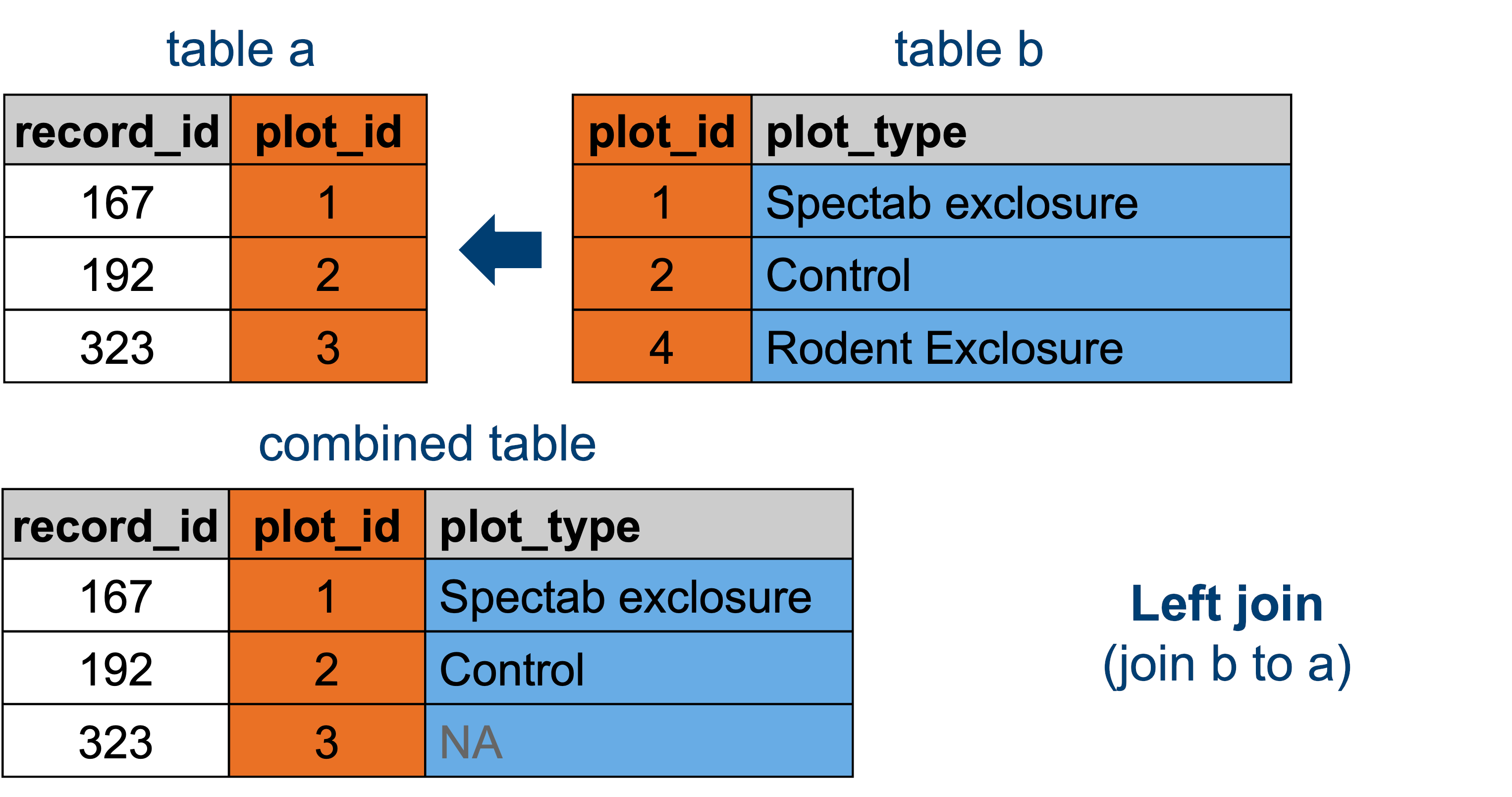
This means that any plot_id that appears in surveys, but isn’t present in plot_types will be empty or missing for its plot_type value.
For an animated representation of the underlying principle of joining, have a look at the garrickadenbuie website.
left_join(surveys, plot_types, by = "plot_id")# A tibble: 35,549 × 10
record_id month day year plot_id species_id sex hindfoot_length weight
<dbl> <dbl> <dbl> <dbl> <dbl> <chr> <chr> <dbl> <dbl>
1 1 7 16 1977 2 NL M 32 NA
2 2 7 16 1977 3 NL M 33 NA
3 3 7 16 1977 2 DM F 37 NA
4 4 7 16 1977 7 DM M 36 NA
5 5 7 16 1977 3 DM M 35 NA
6 6 7 16 1977 1 PF M 14 NA
7 7 7 16 1977 2 PE F NA NA
8 8 7 16 1977 1 DM M 37 NA
9 9 7 16 1977 1 DM F 34 NA
10 10 7 16 1977 6 PF F 20 NA
# ℹ 35,539 more rows
# ℹ 1 more variable: plot_type <chr>Let’s assign that output to an object called surveys_left.
surveys_left <- left_join(surveys, plot_types, by = "plot_id")surveys_left = pd.merge(surveys, plot_types, how = "left", on = "plot_id")surveys_left record_id month ... weight plot_type
0 1 7 ... NaN Control
1 2 7 ... NaN Long-term Krat Exclosure
2 3 7 ... NaN Control
3 4 7 ... NaN NaN
4 5 7 ... NaN Long-term Krat Exclosure
... ... ... ... ... ...
35544 35545 12 ... NaN NaN
35545 35546 12 ... NaN NaN
35546 35547 12 ... 14.0 NaN
35547 35548 12 ... 51.0 NaN
35548 35549 12 ... NaN Short-term Krat Exclosure
[35549 rows x 10 columns]Having this information now allows us to plot the data by plot_type in a much more meaningful way than if we would have used plot_id. For example, let’s look at the hindfoot_length for each plot_type.
ggplot(surveys_left, aes(x = plot_type, y = hindfoot_length)) +
  geom_boxplot()
Warning: Removed 4111 rows containing non-finite outside the scale range
(`stat_boxplot()`).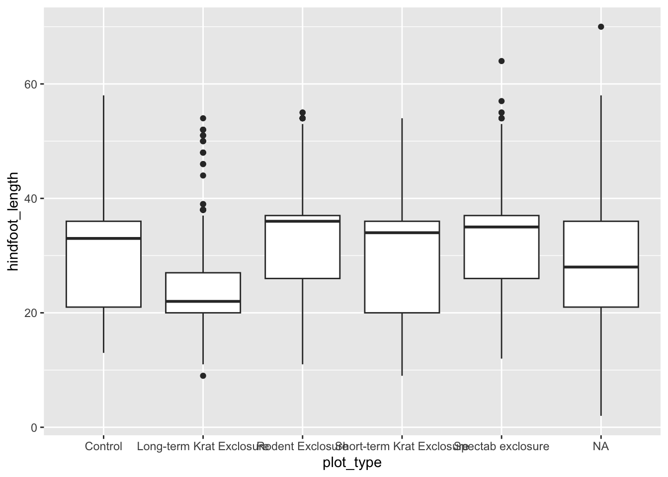
p = (ggplot(surveys_left, aes(x = "plot_type", y = "hindfoot_length")) +
  geom_boxplot())

p.show()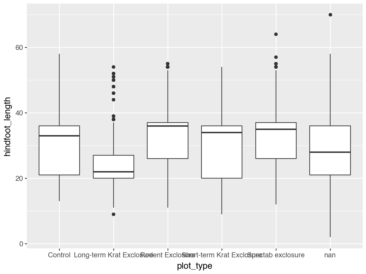
NoteSeaborn equivalent
sns.boxplot(
    data = surveys_left,
    x = "plot_type",
    y = "hindfoot_length"
)

plt.title("Hindfoot length by plot type")
plt.show()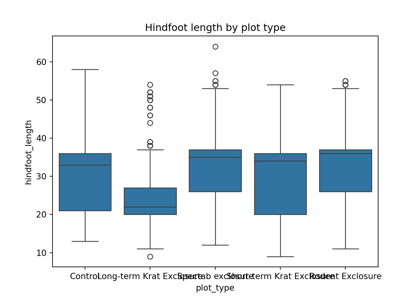
13.3.3 Right joins
Now we’re doing a join in the opposite direction: we’re joining the surveys data set to the plot_types data set. Conceptually, this looks like so:
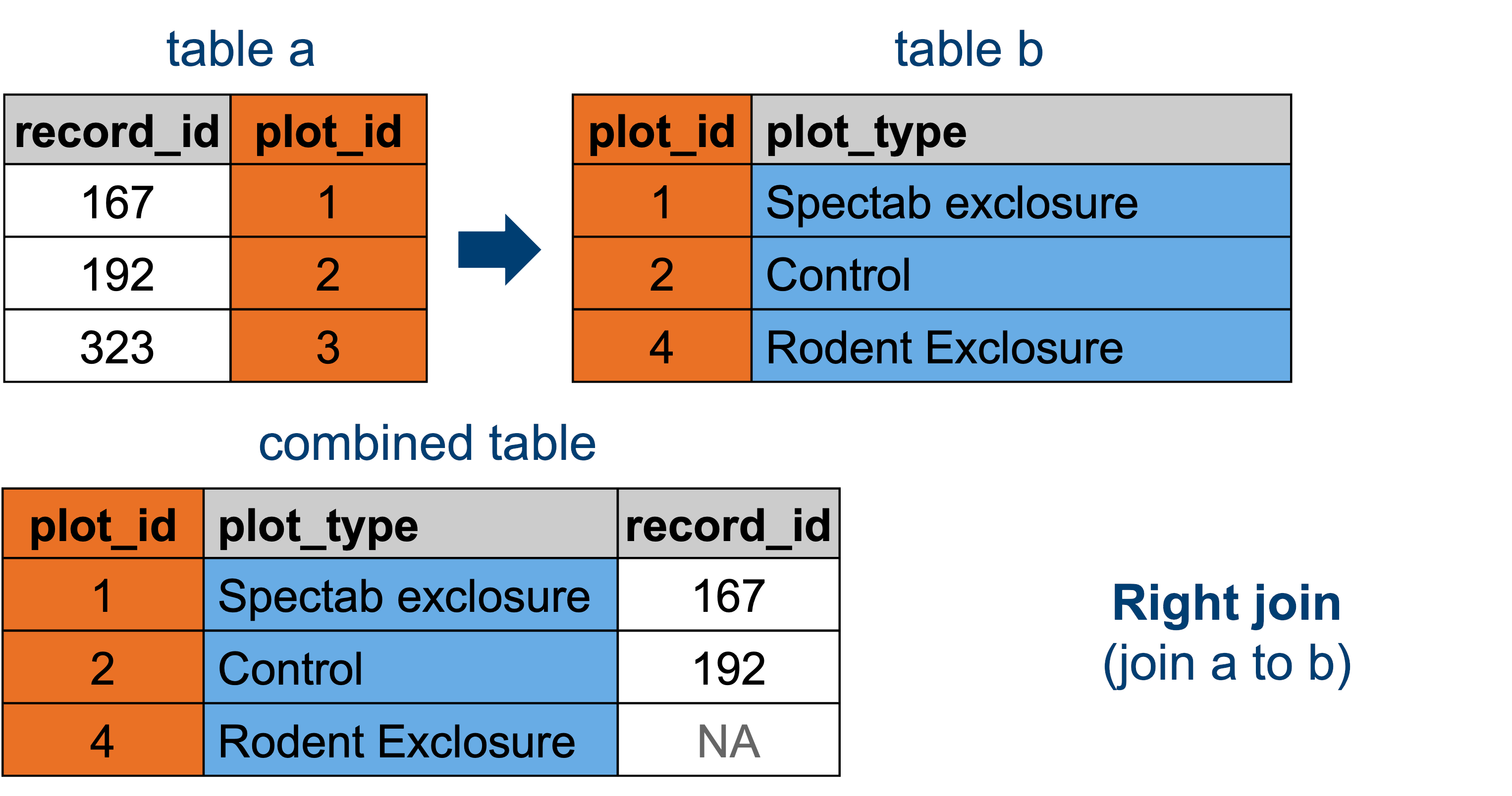
This means that for all the rows where there isn’t a match for plot_id in the surveys data set, the rows are dropped.
right_join(surveys, plot_types, by = "plot_id")# A tibble: 9,180 × 10
record_id month day year plot_id species_id sex hindfoot_length weight
<dbl> <dbl> <dbl> <dbl> <dbl> <chr> <chr> <dbl> <dbl>
1 1 7 16 1977 2 NL M 32 NA
2 2 7 16 1977 3 NL M 33 NA
3 3 7 16 1977 2 DM F 37 NA
4 5 7 16 1977 3 DM M 35 NA
5 6 7 16 1977 1 PF M 14 NA
6 7 7 16 1977 2 PE F NA NA
7 8 7 16 1977 1 DM M 37 NA
8 9 7 16 1977 1 DM F 34 NA
9 11 7 16 1977 5 DS F 53 NA
10 13 7 16 1977 3 DM M 35 NA
# ℹ 9,170 more rows
# ℹ 1 more variable: plot_type <chr>surveys_right = pd.merge(surveys, plot_types, how = "right", on = "plot_id")Let’s see how many rows we’ve retained.
len(surveys_right)9180We can see that we have far fewer rows left (9180) than in the full data set (35549). This is because all the rows where there isn’t a match for plot_id in the surveys data set are dropped.
13.3.4 Inner joins
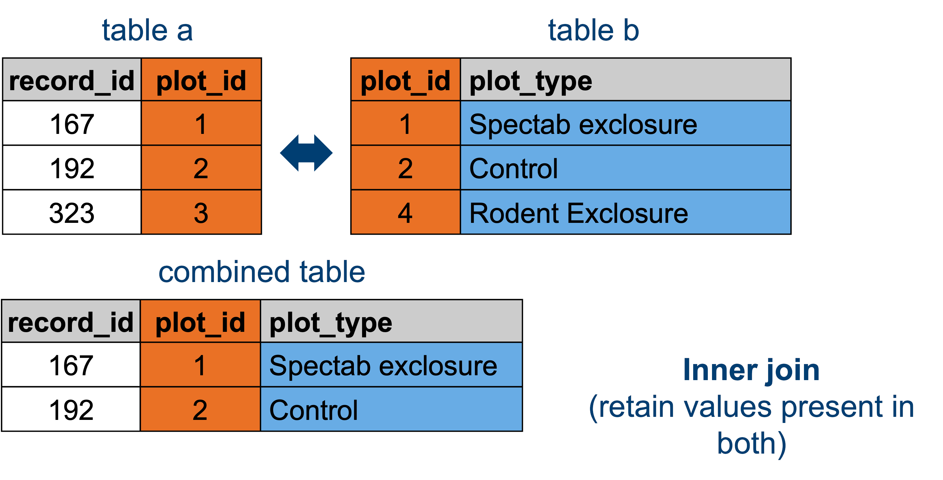
inner_join(surveys, plot_types, by = "plot_id")# A tibble: 9,180 × 10
record_id month day year plot_id species_id sex hindfoot_length weight
<dbl> <dbl> <dbl> <dbl> <dbl> <chr> <chr> <dbl> <dbl>
1 1 7 16 1977 2 NL M 32 NA
2 2 7 16 1977 3 NL M 33 NA
3 3 7 16 1977 2 DM F 37 NA
4 5 7 16 1977 3 DM M 35 NA
5 6 7 16 1977 1 PF M 14 NA
6 7 7 16 1977 2 PE F NA NA
7 8 7 16 1977 1 DM M 37 NA
8 9 7 16 1977 1 DM F 34 NA
9 11 7 16 1977 5 DS F 53 NA
10 13 7 16 1977 3 DM M 35 NA
# ℹ 9,170 more rows
# ℹ 1 more variable: plot_type <chr>surveys_inner = pd.merge(surveys, plot_types, how = "inner", on = "plot_id")Let’s see how many rows we’ve retained. We can either use .shape[0] or len().
len(surveys_inner)9180This actually gives the same result as with the right join (9180 rows), which is because there aren’t any rows in plot_type that don’t have a match in surveys.
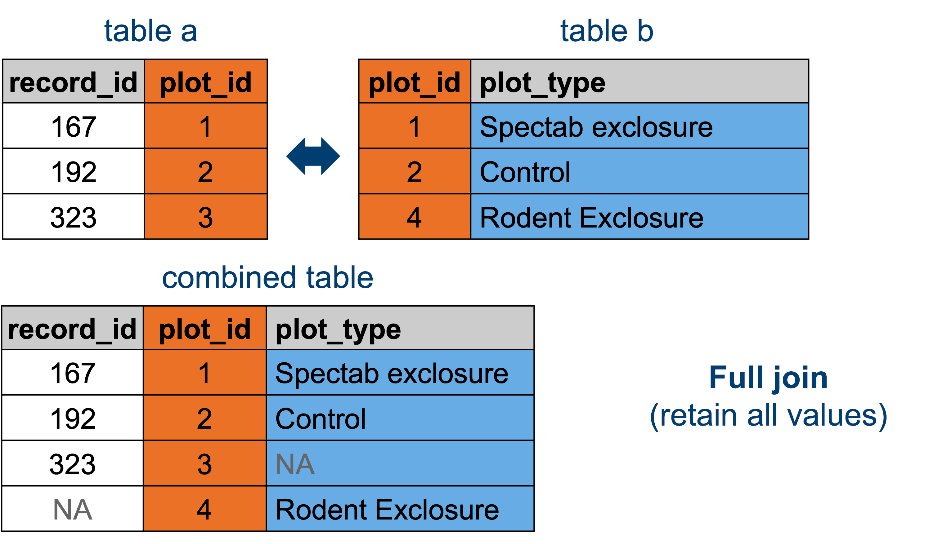
13.3.5 Full joins
full_join(surveys, plot_types, by = "plot_id")# A tibble: 35,549 × 10
record_id month day year plot_id species_id sex hindfoot_length weight
<dbl> <dbl> <dbl> <dbl> <dbl> <chr> <chr> <dbl> <dbl>
1 1 7 16 1977 2 NL M 32 NA
2 2 7 16 1977 3 NL M 33 NA
3 3 7 16 1977 2 DM F 37 NA
4 4 7 16 1977 7 DM M 36 NA
5 5 7 16 1977 3 DM M 35 NA
6 6 7 16 1977 1 PF M 14 NA
7 7 7 16 1977 2 PE F NA NA
8 8 7 16 1977 1 DM M 37 NA
9 9 7 16 1977 1 DM F 34 NA
10 10 7 16 1977 6 PF F 20 NA
# ℹ 35,539 more rows
# ℹ 1 more variable: plot_type <chr>The “full” join in pandas’ merge() function is referred to as "outer".
surveys_full = pd.merge(surveys, plot_types, how = "outer", on = "plot_id")Let’s see how many rows we’ve retained.
len(surveys_full)35549This again gives us our entire surveys data set, including the additional plot_type information where available. The reason why this is not different to the left join is because there are no rows in plot_types that do not have a match in surveys.
13.3.6 Filtering joins
There is one last set of joins we haven’t discussed yet: filtering joins. These can be really helpful if you’re comparing two tables and want to specifically extract the rows that are either present (semi-join) or absent (anti-join) in the other table.
Semi-join:
semi_join(surveys, plot_types, by = "plot_id")# A tibble: 9,180 × 9
record_id month day year plot_id species_id sex hindfoot_length weight
<dbl> <dbl> <dbl> <dbl> <dbl> <chr> <chr> <dbl> <dbl>
1 1 7 16 1977 2 NL M 32 NA
2 2 7 16 1977 3 NL M 33 NA
3 3 7 16 1977 2 DM F 37 NA
4 5 7 16 1977 3 DM M 35 NA
5 6 7 16 1977 1 PF M 14 NA
6 7 7 16 1977 2 PE F NA NA
7 8 7 16 1977 1 DM M 37 NA
8 9 7 16 1977 1 DM F 34 NA
9 11 7 16 1977 5 DS F 53 NA
10 13 7 16 1977 3 DM M 35 NA
# ℹ 9,170 more rowsAnti-join:
anti_join(surveys, plot_types, by = "plot_id")# A tibble: 26,369 × 9
record_id month day year plot_id species_id sex hindfoot_length weight
<dbl> <dbl> <dbl> <dbl> <dbl> <chr> <chr> <dbl> <dbl>
1 4 7 16 1977 7 DM M 36 NA
2 10 7 16 1977 6 PF F 20 NA
3 12 7 16 1977 7 DM M 38 NA
4 14 7 16 1977 8 DM <NA> NA NA
5 15 7 16 1977 6 DM F 36 NA
6 20 7 17 1977 11 DS F 48 NA
7 21 7 17 1977 14 DM F 34 NA
8 22 7 17 1977 15 NL F 31 NA
9 23 7 17 1977 13 DM M 36 NA
10 24 7 17 1977 13 SH M 21 NA
# ℹ 26,359 more rowsSemi-join:
surveys[surveys["plot_id"].isin(plot_types["plot_id"])] record_id month day year ... species_id sex hindfoot_length weight
0 1 7 16 1977 ... NL M 32.0 NaN
1 2 7 16 1977 ... NL M 33.0 NaN
2 3 7 16 1977 ... DM F 37.0 NaN
4 5 7 16 1977 ... DM M 35.0 NaN
5 6 7 16 1977 ... PF M 14.0 NaN
... ... ... ... ... ... ... ... ... ...
35498 35499 12 31 2002 ... PB F 27.0 28.0
35499 35500 12 31 2002 ... PB F 25.0 28.0
35500 35501 12 31 2002 ... DO M 33.0 48.0
35501 35502 12 31 2002 ... PP M 21.0 16.0
35548 35549 12 31 2002 ... NaN NaN NaN NaN
[9180 rows x 9 columns]Anti-join:
surveys[~surveys["plot_id"].isin(plot_types["plot_id"])] record_id month day year ... species_id sex hindfoot_length weight
3 4 7 16 1977 ... DM M 36.0 NaN
9 10 7 16 1977 ... PF F 20.0 NaN
11 12 7 16 1977 ... DM M 38.0 NaN
13 14 7 16 1977 ... DM NaN NaN NaN
14 15 7 16 1977 ... DM F 36.0 NaN
... ... ... ... ... ... ... ... ... ...
35543 35544 12 31 2002 ... US NaN NaN NaN
35544 35545 12 31 2002 ... AH NaN NaN NaN
35545 35546 12 31 2002 ... AH NaN NaN NaN
35546 35547 12 31 2002 ... RM F 15.0 14.0
35547 35548 12 31 2002 ... DO M 36.0 51.0
[26369 rows x 9 columns]13.4 Exercises
13.4.1 Simple joins: surveys
13.5 Summary
TipKey points
- We can use left, right, inner and outer/full joins to merge two tables together.
- There needs to be at least one matching column between the two tables that can be used as a key to link them.
- We can also use filter joins to identify rows in a table that are present/absent in the other