8  Manipulating columns

Learning objectives

• Learn how to select and/or rename specific columns from a data frame.
• Be able to create new columns and modify existing ones.

8.1 Context

In the tabular data section we learned to deal with, well, tabular data in the form of our surveys data set. This data set isn’t huge, but sometimes we have many variables and we might only want to work with a subset of them. Or, we might want to create new columns based on existing data. In this section we’ll cover how we can do this.

8.2 Section setup

Click to expand

R

We’ll continue this section with the script named da3-05-manipulating-columns.R. If needed, add the following code to the top of your script and run it.

# A collection of R packages designed for data science
library(tidyverse)

surveys <- read_csv("data/surveys.csv")

Python

We’ll continue this section with the script named da3-05-manipulating-columns.py. If needed, add the following code to the top of your script and run it.

# A Python data analysis and manipulation tool
import pandas as pd

# Python equivalent of `ggplot2`
from plotnine import *

surveys = pd.read_csv("data/surveys.csv")

8.3 Selecting columns

Let’s remind ourselves to which columns we have in our surveys data set. After that, we’ll start making some changes.

R

colnames(surveys)

[1] "record_id"       "month"           "day"             "year"           
[5] "plot_id"         "species_id"      "sex"             "hindfoot_length"
[9] "weight"         

Python

surveys.columns

Index(['record_id', 'month', 'day', 'year', 'plot_id', 'species_id', 'sex',
       'hindfoot_length', 'weight'],
      dtype='object')

8.3.1 Selecting individual columns

Let’s say we wanted to select only the record_id and year columns. We’ve briefly done this when we looked at subsetting rows and columns.

R

However, there is an alternative way of doing this using the dplyr package - which is part of tidyverse.

We can use the select() function:

select(surveys, record_id, year)

# A tibble: 35,549 × 2
   record_id  year
       <dbl> <dbl>
 1         1  1977
 2         2  1977
 3         3  1977
 4         4  1977
 5         5  1977
 6         6  1977
 7         7  1977
 8         8  1977
 9         9  1977
10        10  1977
# ℹ 35,539 more rows

Using the base R syntax, this is equivalent to surveys[, c("record_id", "year")]. Notice that with the select() function (and generally with dplyr functions) we didn’t need to quote ” the column names. This is because the first input to the function is the table name, and so everything after is assumed to be column names of that table.

Python

The way we need to specify this is by giving a list of column names ["record_id", "year"] and subsetting the surveys data set with this.

The way we subset is with surveys[ ], so we end up with double square brackets:

surveys[["record_id", "year"]]

       record_id  year
0              1  1977
1              2  1977
2              3  1977
3              4  1977
4              5  1977
...          ...   ...
35544      35545  2002
35545      35546  2002
35546      35547  2002
35547      35548  2002
35548      35549  2002

[35549 rows x 2 columns]

8.3.2 Selecting with helper functions

R

The select() function becomes particularly useful when we combine it with other helper functions. For example, this code will select all the columns where the column name contains the string (text) "_id":

# returns all columns where the column name contains the text "_id"
select(surveys, contains("_id"))

# A tibble: 35,549 × 3
   record_id plot_id species_id
       <dbl>   <dbl> <chr>     
 1         1       2 NL        
 2         2       3 NL        
 3         3       2 DM        
 4         4       7 DM        
 5         5       3 DM        
 6         6       1 PF        
 7         7       2 PE        
 8         8       1 DM        
 9         9       1 DM        
10        10       6 PF        
# ℹ 35,539 more rows

Another thing we often want to do is select columns by their data type. For example, if we wanted to select all numerical columns we could do this:

select(surveys, where(is.numeric))

# A tibble: 35,549 × 7
   record_id month   day  year plot_id hindfoot_length weight
       <dbl> <dbl> <dbl> <dbl>   <dbl>           <dbl>  <dbl>
 1         1     7    16  1977       2              32     NA
 2         2     7    16  1977       3              33     NA
 3         3     7    16  1977       2              37     NA
 4         4     7    16  1977       7              36     NA
 5         5     7    16  1977       3              35     NA
 6         6     7    16  1977       1              14     NA
 7         7     7    16  1977       2              NA     NA
 8         8     7    16  1977       1              37     NA
 9         9     7    16  1977       1              34     NA
10        10     7    16  1977       6              20     NA
# ℹ 35,539 more rows

Python

The subsetting becomes a bit tedious when we’re looking for patterns in the column names. Here, we can instead use the .filter attribute of the surveys data set, and look for a string (text) where the column name contains "_id".

surveys.filter(like = "_id")

       record_id  plot_id species_id
0              1        2         NL
1              2        3         NL
2              3        2         DM
3              4        7         DM
4              5        3         DM
...          ...      ...        ...
35544      35545       15         AH
35545      35546       15         AH
35546      35547       10         RM
35547      35548        7         DO
35548      35549        5        NaN

[35549 rows x 3 columns]

Another thing we often want to do is select columns by their data type. For example, if we wanted to select all numerical columns we could do this:

surveys.select_dtypes(include = ["number"])

       record_id  month  day  year  plot_id  hindfoot_length  weight
0              1      7   16  1977        2             32.0     NaN
1              2      7   16  1977        3             33.0     NaN
2              3      7   16  1977        2             37.0     NaN
3              4      7   16  1977        7             36.0     NaN
4              5      7   16  1977        3             35.0     NaN
...          ...    ...  ...   ...      ...              ...     ...
35544      35545     12   31  2002       15              NaN     NaN
35545      35546     12   31  2002       15              NaN     NaN
35546      35547     12   31  2002       10             15.0    14.0
35547      35548     12   31  2002        7             36.0    51.0
35548      35549     12   31  2002        5              NaN     NaN

[35549 rows x 7 columns]

8.3.3 Selecting a range of columns

Let’s say we’re interested in all the columns from record_id to year.

R

In that case, we can use the : symbol.

# returns all columns between and including record_id and year
select(surveys, record_id:year)

# A tibble: 35,549 × 4
   record_id month   day  year
       <dbl> <dbl> <dbl> <dbl>
 1         1     7    16  1977
 2         2     7    16  1977
 3         3     7    16  1977
 4         4     7    16  1977
 5         5     7    16  1977
 6         6     7    16  1977
 7         7     7    16  1977
 8         8     7    16  1977
 9         9     7    16  1977
10        10     7    16  1977
# ℹ 35,539 more rows

We can also combine this with the previous method:

# returns all columns between and including record_id and year
# and all columns where the column name contains the text "_id"
select(surveys, record_id:year, contains("_id"))

# A tibble: 35,549 × 6
   record_id month   day  year plot_id species_id
       <dbl> <dbl> <dbl> <dbl>   <dbl> <chr>     
 1         1     7    16  1977       2 NL        
 2         2     7    16  1977       3 NL        
 3         3     7    16  1977       2 DM        
 4         4     7    16  1977       7 DM        
 5         5     7    16  1977       3 DM        
 6         6     7    16  1977       1 PF        
 7         7     7    16  1977       2 PE        
 8         8     7    16  1977       1 DM        
 9         9     7    16  1977       1 DM        
10        10     7    16  1977       6 PF        
# ℹ 35,539 more rows

Python

In that case, we can use the : symbol, in combination with the .loc indexer.

surveys.loc[:, "record_id":"year"]

       record_id  month  day  year
0              1      7   16  1977
1              2      7   16  1977
2              3      7   16  1977
3              4      7   16  1977
4              5      7   16  1977
...          ...    ...  ...   ...
35544      35545     12   31  2002
35545      35546     12   31  2002
35546      35547     12   31  2002
35547      35548     12   31  2002
35548      35549     12   31  2002

[35549 rows x 4 columns]

8.3.4 Unselecting columns

Lastly, we can also unselect columns. This can be useful when you want most columns, apart from some.

R

To do this, we use the - symbol before the column name.

# returns all columns apart from record_id
select(surveys, -record_id)

# A tibble: 35,549 × 8
   month   day  year plot_id species_id sex   hindfoot_length weight
   <dbl> <dbl> <dbl>   <dbl> <chr>      <chr>           <dbl>  <dbl>
 1     7    16  1977       2 NL         M                  32     NA
 2     7    16  1977       3 NL         M                  33     NA
 3     7    16  1977       2 DM         F                  37     NA
 4     7    16  1977       7 DM         M                  36     NA
 5     7    16  1977       3 DM         M                  35     NA
 6     7    16  1977       1 PF         M                  14     NA
 7     7    16  1977       2 PE         F                  NA     NA
 8     7    16  1977       1 DM         M                  37     NA
 9     7    16  1977       1 DM         F                  34     NA
10     7    16  1977       6 PF         F                  20     NA
# ℹ 35,539 more rows

Python

To do this, we use the .drop attribute. Here, we only unselect one column, but we can easily extend this by providing a list of columns do the column = argument.

surveys.drop(columns = "record_id")

       month  day  year  plot_id species_id  sex  hindfoot_length  weight
0          7   16  1977        2         NL    M             32.0     NaN
1          7   16  1977        3         NL    M             33.0     NaN
2          7   16  1977        2         DM    F             37.0     NaN
3          7   16  1977        7         DM    M             36.0     NaN
4          7   16  1977        3         DM    M             35.0     NaN
...      ...  ...   ...      ...        ...  ...              ...     ...
35544     12   31  2002       15         AH  NaN              NaN     NaN
35545     12   31  2002       15         AH  NaN              NaN     NaN
35546     12   31  2002       10         RM    F             15.0    14.0
35547     12   31  2002        7         DO    M             36.0    51.0
35548     12   31  2002        5        NaN  NaN              NaN     NaN

[35549 rows x 8 columns]

8.4 Renaming and reshuffling columns

8.4.1 Renaming columns

For example, we might want to change the weight column name to weight_g, to reflect that the values are in grams.

R

We can use the rename() function to change a column name. We do this as follows:

rename(surveys, weight_g = weight)

# A tibble: 35,549 × 9
   record_id month   day  year plot_id species_id sex   hindfoot_length weight_g
       <dbl> <dbl> <dbl> <dbl>   <dbl> <chr>      <chr>           <dbl>    <dbl>
 1         1     7    16  1977       2 NL         M                  32       NA
 2         2     7    16  1977       3 NL         M                  33       NA
 3         3     7    16  1977       2 DM         F                  37       NA
 4         4     7    16  1977       7 DM         M                  36       NA
 5         5     7    16  1977       3 DM         M                  35       NA
 6         6     7    16  1977       1 PF         M                  14       NA
 7         7     7    16  1977       2 PE         F                  NA       NA
 8         8     7    16  1977       1 DM         M                  37       NA
 9         9     7    16  1977       1 DM         F                  34       NA
10        10     7    16  1977       6 PF         F                  20       NA
# ℹ 35,539 more rows

Python

We can use the .rename() attribute of the surveys pandas DataFrame:

surveys.rename(columns = {'weight': 'weight_g'})

       record_id  month  day  year  ...  species_id  sex hindfoot_length  weight_g
0              1      7   16  1977  ...          NL    M            32.0       NaN
1              2      7   16  1977  ...          NL    M            33.0       NaN
2              3      7   16  1977  ...          DM    F            37.0       NaN
3              4      7   16  1977  ...          DM    M            36.0       NaN
4              5      7   16  1977  ...          DM    M            35.0       NaN
...          ...    ...  ...   ...  ...         ...  ...             ...       ...
35544      35545     12   31  2002  ...          AH  NaN             NaN       NaN
35545      35546     12   31  2002  ...          AH  NaN             NaN       NaN
35546      35547     12   31  2002  ...          RM    F            15.0      14.0
35547      35548     12   31  2002  ...          DO    M            36.0      51.0
35548      35549     12   31  2002  ...         NaN  NaN             NaN       NaN

[35549 rows x 9 columns]

8.4.2 Reshuffling columns

It might be that you want to reorder/reshuffle a column. Here, the year column is our fourth variable. Let’s say we’d want to move this to the second position (after record_id).

R

We can use the relocate() function to do this. The function has several arguments, starting with ., such as .before = or .after =. These allow you to specify where you want to reinsert the column.

relocate(surveys, year, .after = record_id)

# A tibble: 35,549 × 9
   record_id  year month   day plot_id species_id sex   hindfoot_length weight
       <dbl> <dbl> <dbl> <dbl>   <dbl> <chr>      <chr>           <dbl>  <dbl>
 1         1  1977     7    16       2 NL         M                  32     NA
 2         2  1977     7    16       3 NL         M                  33     NA
 3         3  1977     7    16       2 DM         F                  37     NA
 4         4  1977     7    16       7 DM         M                  36     NA
 5         5  1977     7    16       3 DM         M                  35     NA
 6         6  1977     7    16       1 PF         M                  14     NA
 7         7  1977     7    16       2 PE         F                  NA     NA
 8         8  1977     7    16       1 DM         M                  37     NA
 9         9  1977     7    16       1 DM         F                  34     NA
10        10  1977     7    16       6 PF         F                  20     NA
# ℹ 35,539 more rows

Python

Unlike in R, there isn’t a very clear, straightforward way of reinserting columns in a pandas DataFrame. We could show you convoluted ways of doing so, but at this point that’s just confusing. So, we’ll leave you with a link to a Stackoverflow solution.

8.5 Creating new columns

Sometimes we need to create new columns. For example, we might have a variable that is not in the unit of measurement we need (e.g. in millimeters, instead of centimeters).

Conceptually, that looks something like this:

Figure 8.1: Creating a new column using data from an existing one.

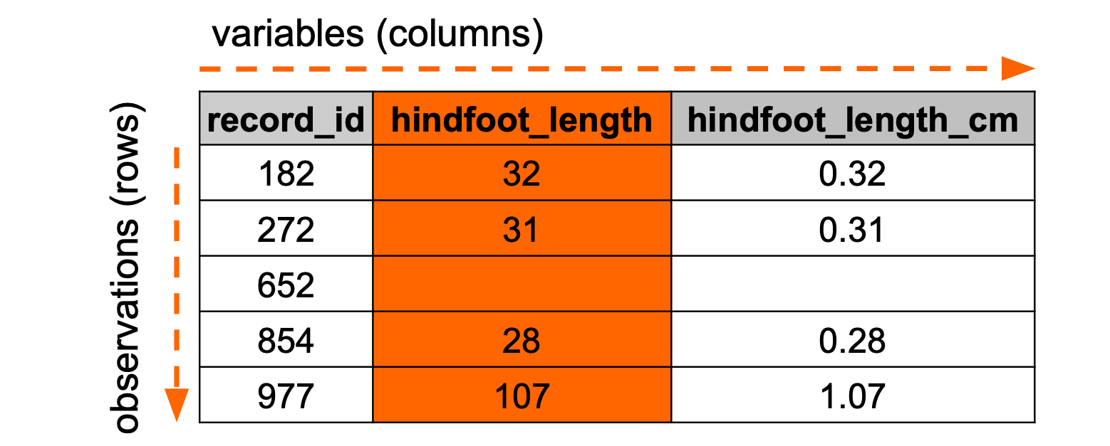
Let’s illustrate this with an example on our surveys data set. Let’s say we wanted to get hindfoot_length in centimeters, instead of millimeters. We’d have to go through each row, take the hindfoot_length value and divide it by 10. We then need to store this output in a column called, for example, hindfoot_length_cm.

R

We can use the mutate() function to create new columns:

mutate(surveys, hindfoot_length_cm = hindfoot_length / 10)

# A tibble: 35,549 × 10
   record_id month   day  year plot_id species_id sex   hindfoot_length weight
       <dbl> <dbl> <dbl> <dbl>   <dbl> <chr>      <chr>           <dbl>  <dbl>
 1         1     7    16  1977       2 NL         M                  32     NA
 2         2     7    16  1977       3 NL         M                  33     NA
 3         3     7    16  1977       2 DM         F                  37     NA
 4         4     7    16  1977       7 DM         M                  36     NA
 5         5     7    16  1977       3 DM         M                  35     NA
 6         6     7    16  1977       1 PF         M                  14     NA
 7         7     7    16  1977       2 PE         F                  NA     NA
 8         8     7    16  1977       1 DM         M                  37     NA
 9         9     7    16  1977       1 DM         F                  34     NA
10        10     7    16  1977       6 PF         F                  20     NA
# ℹ 35,539 more rows
# ℹ 1 more variable: hindfoot_length_cm <dbl>

Python

We use the square brackets to define the name of the new column, then specify what needs to go in the new column:

surveys['hindfoot_length_cm'] = surveys['hindfoot_length'] / 10

Although it has created the column, we can’t quite see it because we have too many columns. So, let’s save the new column to the data set and then select the relevant columns.

R

First, we update our data:

surveys <- mutate(surveys, hindfoot_length_cm = hindfoot_length / 10)

Next, we can select the columns.

select(surveys, record_id, hindfoot_length, hindfoot_length_cm)

# A tibble: 35,549 × 3
   record_id hindfoot_length hindfoot_length_cm
       <dbl>           <dbl>              <dbl>
 1         1              32                3.2
 2         2              33                3.3
 3         3              37                3.7
 4         4              36                3.6
 5         5              35                3.5
 6         6              14                1.4
 7         7              NA               NA  
 8         8              37                3.7
 9         9              34                3.4
10        10              20                2  
# ℹ 35,539 more rows

Python

Our previous step already added the new column to the DataFrame, so we can directly select the relevant columns, by giving a list of the columns we’re interested in:

surveys[['record_id', 'hindfoot_length', 'hindfoot_length_cm']]

       record_id  hindfoot_length  hindfoot_length_cm
0              1             32.0                 3.2
1              2             33.0                 3.3
2              3             37.0                 3.7
3              4             36.0                 3.6
4              5             35.0                 3.5
...          ...              ...                 ...
35544      35545              NaN                 NaN
35545      35546              NaN                 NaN
35546      35547             15.0                 1.5
35547      35548             36.0                 3.6
35548      35549              NaN                 NaN

[35549 rows x 3 columns]

We can see that each value in hindfoot_length_cm is a tenth of the value of hindfoot_length. This is exactly what we expected!

8.6 Exercises

8.6.1 Selecting columns: infections

Exercise 1 - Selecting columns

Level:

For this exercise we’ll be using a new data set, called infections. These are synthetic data (see the script if you would like to know more).

Please do the following:

1. Read in the data
2. Get to grips with the structure of the data
3. Select the patient_id, systolic_pressure and body_temperature columns
4. Select all numerical columns
5. Unselect all logical columns

Answer

1. Read in the data

First we load the data, and have a glimpse of it.

R

infections <- read_csv("data/infections.csv")

head(infections)

# A tibble: 6 × 11
  patient_id hospital   quarter infection_type vaccination_status age_group
  <chr>      <chr>      <chr>   <chr>          <chr>              <chr>    
1 ID_0001    hospital_3 Q2      none           <NA>               65+      
2 ID_0002    hospital_3 Q2      viral          <NA>               18 - 64  
3 ID_0003    hospital_2 Q2      none           unknown            65+      
4 ID_0004    hospital_2 Q3      fungal         unvaccinated       < 18     
5 ID_0005    hospital_3 Q2      fungal         vaccinated         65+      
6 ID_0006    hospital_5 Q3      none           vaccinated         65+      
# ℹ 5 more variables: icu_admission <lgl>, symptoms_count <dbl>,
#   systolic_pressure <dbl>, body_temperature <dbl>, crp_level <dbl>

Python

infections = pd.read_csv("data/infections.csv")

infections.head()

  patient_id    hospital  ... body_temperature crp_level
0    ID_0001  hospital_3  ...             37.8     12.05
1    ID_0002  hospital_3  ...             39.1      8.11
2    ID_0003  hospital_2  ...             38.5      5.24
3    ID_0004  hospital_2  ...             39.4     41.73
4    ID_0005  hospital_3  ...             36.9     10.51

[5 rows x 11 columns]

2. Get to grips with the structure of the data

Before delving into any analysis, it’s always good to have a good look at your data, so you know what you’re dealing with. We can look at the overall structure (focussing on the column types & checking if they make sense), at number of columns/observations, column names, summary statistics etc.

R

str(infections) # overall structure

spc_tbl_ [1,400 × 11] (S3: spec_tbl_df/tbl_df/tbl/data.frame)
 $ patient_id        : chr [1:1400] "ID_0001" "ID_0002" "ID_0003" "ID_0004" ...
 $ hospital          : chr [1:1400] "hospital_3" "hospital_3" "hospital_2" "hospital_2" ...
 $ quarter           : chr [1:1400] "Q2" "Q2" "Q2" "Q3" ...
 $ infection_type    : chr [1:1400] "none" "viral" "none" "fungal" ...
 $ vaccination_status: chr [1:1400] NA NA "unknown" "unvaccinated" ...
 $ age_group         : chr [1:1400] "65+" "18 - 64" "65+" "< 18" ...
 $ icu_admission     : logi [1:1400] FALSE FALSE TRUE TRUE TRUE FALSE ...
 $ symptoms_count    : num [1:1400] 1 6 3 7 7 5 10 12 13 7 ...
 $ systolic_pressure : num [1:1400] 117 115 120 129 114 124 133 120 124 127 ...
 $ body_temperature  : num [1:1400] 37.8 39.1 38.5 39.4 36.9 36.8 39.4 39.3 39.6 39.1 ...
 $ crp_level         : num [1:1400] 12.05 8.11 5.24 41.73 10.51 ...
 - attr(*, "spec")=
  .. cols(
  ..   patient_id = col_character(),
  ..   hospital = col_character(),
  ..   quarter = col_character(),
  ..   infection_type = col_character(),
  ..   vaccination_status = col_character(),
  ..   age_group = col_character(),
  ..   icu_admission = col_logical(),
  ..   symptoms_count = col_double(),
  ..   systolic_pressure = col_double(),
  ..   body_temperature = col_double(),
  ..   crp_level = col_double()
  .. )
 - attr(*, "problems")=<externalptr> 

nrow(infections) # row number

[1] 1400

ncol(infections) # column number

[1] 11

colnames(infections) # column names

 [1] "patient_id"         "hospital"           "quarter"           
 [4] "infection_type"     "vaccination_status" "age_group"         
 [7] "icu_admission"      "symptoms_count"     "systolic_pressure" 
[10] "body_temperature"   "crp_level"         

summary(infections) # summary statistics

  patient_id          hospital           quarter          infection_type    
 Length:1400        Length:1400        Length:1400        Length:1400       
 Class :character   Class :character   Class :character   Class :character  
 Mode  :character   Mode  :character   Mode  :character   Mode  :character  
                                                                            
                                                                            
                                                                            
                                                                            
 vaccination_status  age_group         icu_admission   symptoms_count  
 Length:1400        Length:1400        Mode :logical   Min.   : 0.000  
 Class :character   Class :character   FALSE:814       1st Qu.: 6.000  
 Mode  :character   Mode  :character   TRUE :513       Median : 9.000  
                                       NA's :73        Mean   : 8.549  
                                                       3rd Qu.:11.000  
                                                       Max.   :21.000  
                                                       NA's   :67      
 systolic_pressure body_temperature   crp_level     
 Min.   : 87.0     Min.   :36.30    Min.   : 1.000  
 1st Qu.:118.0     1st Qu.:38.20    1st Qu.: 9.117  
 Median :125.0     Median :38.80    Median :16.215  
 Mean   :125.1     Mean   :38.75    Mean   :19.465  
 3rd Qu.:132.0     3rd Qu.:39.40    3rd Qu.:26.433  
 Max.   :163.0     Max.   :41.50    Max.   :58.860  
 NA's   :74        NA's   :67       NA's   :156     

Python

infections.info() # overall structure

<class 'pandas.core.frame.DataFrame'>
RangeIndex: 1400 entries, 0 to 1399
Data columns (total 11 columns):
 #   Column              Non-Null Count  Dtype  
---  ------              --------------  -----  
 0   patient_id          1400 non-null   object 
 1   hospital            1332 non-null   object 
 2   quarter             1325 non-null   object 
 3   infection_type      1326 non-null   object 
 4   vaccination_status  1325 non-null   object 
 5   age_group           1329 non-null   object 
 6   icu_admission       1327 non-null   object 
 7   symptoms_count      1333 non-null   float64
 8   systolic_pressure   1326 non-null   float64
 9   body_temperature    1333 non-null   float64
 10  crp_level           1244 non-null   float64
dtypes: float64(4), object(7)
memory usage: 120.4+ KB

infections.shape[0] # row number

1400

infections.shape[1] # column number

11

infections.columns # column names

Index(['patient_id', 'hospital', 'quarter', 'infection_type',
       'vaccination_status', 'age_group', 'icu_admission', 'symptoms_count',
       'systolic_pressure', 'body_temperature', 'crp_level'],
      dtype='object')

infections.describe() # summary statistics

       symptoms_count  systolic_pressure  body_temperature    crp_level
count     1333.000000        1326.000000       1333.000000  1244.000000
mean         8.549137         125.070136         38.751988    19.464751
std          3.825004          10.346761          0.883689    13.083907
min          0.000000          87.000000         36.300000     1.000000
25%          6.000000         118.000000         38.200000     9.117500
50%          9.000000         125.000000         38.800000    16.215000
75%         11.000000         132.000000         39.400000    26.432500
max         21.000000         163.000000         41.500000    58.860000

Now that we have a much better view of what our data looks like, let’s play around with selecting and manipulating columns.

3. Select the patient_id, systolic_pressure and body_temperature columns

R

select(infections, patient_id, systolic_pressure, body_temperature)

# A tibble: 1,400 × 3
   patient_id systolic_pressure body_temperature
   <chr>                  <dbl>            <dbl>
 1 ID_0001                  117             37.8
 2 ID_0002                  115             39.1
 3 ID_0003                  120             38.5
 4 ID_0004                  129             39.4
 5 ID_0005                  114             36.9
 6 ID_0006                  124             36.8
 7 ID_0007                  133             39.4
 8 ID_0008                  120             39.3
 9 ID_0009                  124             39.6
10 ID_0010                  127             39.1
# ℹ 1,390 more rows

Python

We use the [[ ]] notations, because we are subsetting the DataFrame (infections[ ]) and we are subsetting it by using a list of column names ["patient_id", "systolic_pressure", "body_temperature"]:

infections[["patient_id", "systolic_pressure", "body_temperature"]]

     patient_id  systolic_pressure  body_temperature
0       ID_0001              117.0              37.8
1       ID_0002              115.0              39.1
2       ID_0003              120.0              38.5
3       ID_0004              129.0              39.4
4       ID_0005              114.0              36.9
...         ...                ...               ...
1395    ID_1396              118.0              39.0
1396    ID_1397              117.0              38.8
1397    ID_1398              137.0               NaN
1398    ID_1399              135.0              38.8
1399    ID_1400              129.0              37.0

[1400 rows x 3 columns]

4. Select all numerical columns

R

select(infections, where(is.numeric))

# A tibble: 1,400 × 4
   symptoms_count systolic_pressure body_temperature crp_level
            <dbl>             <dbl>            <dbl>     <dbl>
 1              1               117             37.8     12.0 
 2              6               115             39.1      8.11
 3              3               120             38.5      5.24
 4              7               129             39.4     41.7 
 5              7               114             36.9     10.5 
 6              5               124             36.8      6.57
 7             10               133             39.4     53.1 
 8             12               120             39.3     NA   
 9             13               124             39.6     50.3 
10              7               127             39.1     13.0 
# ℹ 1,390 more rows

Python

infections.select_dtypes(include = ["number"])

      symptoms_count  systolic_pressure  body_temperature  crp_level
0                1.0              117.0              37.8      12.05
1                6.0              115.0              39.1       8.11
2                3.0              120.0              38.5       5.24
3                7.0              129.0              39.4      41.73
4                7.0              114.0              36.9      10.51
...              ...                ...               ...        ...
1395             8.0              118.0              39.0      10.14
1396             3.0              117.0              38.8      34.42
1397             3.0              137.0               NaN      17.30
1398             5.0              135.0              38.8      18.41
1399             3.0              129.0              37.0       7.69

[1400 rows x 4 columns]

5. Unselect all logical columns

R

We can do something similar as with the numerical column, just specifying the logical type and then negating it:

select(infections, -where(is.logical))

# A tibble: 1,400 × 10
   patient_id hospital   quarter infection_type vaccination_status age_group
   <chr>      <chr>      <chr>   <chr>          <chr>              <chr>    
 1 ID_0001    hospital_3 Q2      none           <NA>               65+      
 2 ID_0002    hospital_3 Q2      viral          <NA>               18 - 64  
 3 ID_0003    hospital_2 Q2      none           unknown            65+      
 4 ID_0004    hospital_2 Q3      fungal         unvaccinated       < 18     
 5 ID_0005    hospital_3 Q2      fungal         vaccinated         65+      
 6 ID_0006    hospital_5 Q3      none           vaccinated         65+      
 7 ID_0007    hospital_4 Q1      fungal         unvaccinated       18 - 64  
 8 ID_0008    hospital_1 Q1      <NA>           unvaccinated       18 - 64  
 9 ID_0009    hospital_2 Q1      viral          <NA>               65+      
10 ID_0010    hospital_3 Q3      none           unvaccinated       <NA>     
# ℹ 1,390 more rows
# ℹ 4 more variables: symptoms_count <dbl>, systolic_pressure <dbl>,
#   body_temperature <dbl>, crp_level <dbl>

Python

We can do something similar as with the numerical column, just specifying the bool type and now excluding it:

infections.select_dtypes(exclude = ["bool"])

     patient_id    hospital  ... body_temperature crp_level
0       ID_0001  hospital_3  ...             37.8     12.05
1       ID_0002  hospital_3  ...             39.1      8.11
2       ID_0003  hospital_2  ...             38.5      5.24
3       ID_0004  hospital_2  ...             39.4     41.73
4       ID_0005  hospital_3  ...             36.9     10.51
...         ...         ...  ...              ...       ...
1395    ID_1396  hospital_3  ...             39.0     10.14
1396    ID_1397  hospital_3  ...             38.8     34.42
1397    ID_1398  hospital_1  ...              NaN     17.30
1398    ID_1399  hospital_2  ...             38.8     18.41
1399    ID_1400  hospital_2  ...             37.0      7.69

[1400 rows x 11 columns]

8.6.2 Creating columns: body_temperature_f

Exercise 2 - Creating columns

Level:

For this exercise we’ll again use the data from data/infections.csv. We’ll assume you’ve still have it read in. Please try the following:

Create a body_temperature_f that contains the body temperature measurements in Fahrenheit.

Hint

To convert Celsius to Fahrenheit, do the following:

\[ F = \left( C \times \frac{9}{5} \right) + 32 \]

Answer

We need to update the existing table, so we view the result.

R

infections <- mutate(infections, body_temperature_f = body_temperature * (9/5) + 32)

Let’s check if the result is what we expected.

select(infections, body_temperature, body_temperature_f)

# A tibble: 1,400 × 2
   body_temperature body_temperature_f
              <dbl>              <dbl>
 1             37.8              100. 
 2             39.1              102. 
 3             38.5              101. 
 4             39.4              103. 
 5             36.9               98.4
 6             36.8               98.2
 7             39.4              103. 
 8             39.3              103. 
 9             39.6              103. 
10             39.1              102. 
# ℹ 1,390 more rows

Python

infections["body_temperature_f"] = infections["body_temperature"] * (9/5) + 32

Let’s check if the result is what we expected.

infections[["body_temperature", "body_temperature_f"]]

      body_temperature  body_temperature_f
0                 37.8              100.04
1                 39.1              102.38
2                 38.5              101.30
3                 39.4              102.92
4                 36.9               98.42
...                ...                 ...
1395              39.0              102.20
1396              38.8              101.84
1397               NaN                 NaN
1398              38.8              101.84
1399              37.0               98.60

[1400 rows x 2 columns]

8.6.3 Creating and plotting columns

Exercise 3 - Creating and plotting columns

Level:

We’ll again use the infections data set, but this time we want you to fix the code below to recreate the image. To do so, please change all the <FIXME> entries to the correct code.

R

# create the column for the y-axis values
infections <- mutate(infections, systolic_pressure_kpa = <FIXME> / 7.5006)

# plot the data
ggplot(infections, aes(x = <FIXME>, y = systolic_pressure_kpa)) +
  geom_<FIXME>(aes(fill = <FIXME>))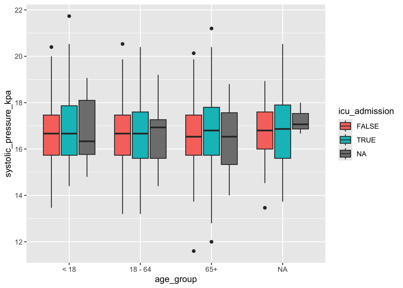

Python

# create the column for the y-axis values
infections["systolic_pressure_kpa"] = infections["<FIXME>"] / 7.5006

# plot the data
p = (ggplot(infections, aes(x = "<FIXME>", y = "systolic_pressure_kpa")) +
  geom_<FIXME>(aes(fill = "<FIXME>")))
  
p.show()

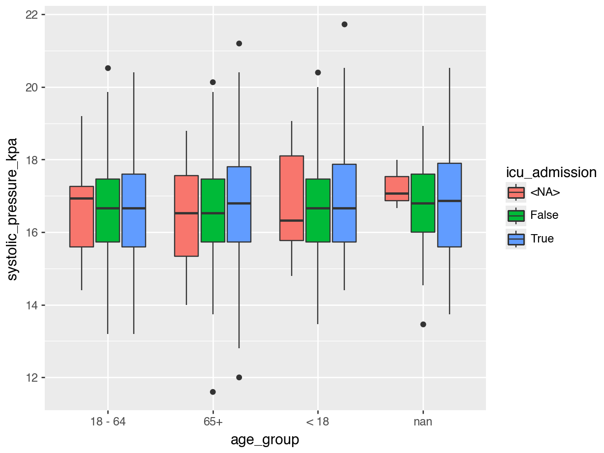
mmHg to kPa

\[ 1\ \text{kPa} \approx 7.5006\ \text{mmHg} \]

Answer

R

# create the column for the y-axis values
infections <- mutate(infections,
                     systolic_pressure_kpa = systolic_pressure / 7.5006)

# plot the data
ggplot(infections, aes(x = age_group, y = systolic_pressure_kpa)) +
  geom_boxplot(aes(fill = icu_admission))

Python

# create the column for the y-axis values
infections["systolic_pressure_kpa"] = infections["systolic_pressure"] / 7.5006

# plot the data
p = (ggplot(infections, aes(x = "age_group", y = "systolic_pressure_kpa")) +
  geom_boxplot(aes(fill = "icu_admission")))
  
p.show()

8.7 Summary

Key points

• We have several functions available that allow us to select, move, rename and create new columns