# A collection of R packages designed for data science
library(tidyverse)

surveys <- read_csv("data/surveys.csv")
infections <- read_csv("data/infections.csv")11 Grouped operations
TipLearning objectives
- Learn how to use grouped operations in data analysis.
- Be able to distinguish between grouped summaries and other types of grouped operations.
11.1 Context
We’ve done different types of operations, all on the entire data set. Sometimes there is structure within the data, such as different groups (e.g. genotypes, patient cohorts, geographical areas etc). We might then want information on a group-by-group basis.
11.2 Section setup
We’ll continue this section with the script named 03_session. If needed, add the following code to the top of your script and run it.
We’ll continue this section with the Notebook named 03_session. Add the following code to the first cell and run it.
# A Python data analysis and manipulation tool
import pandas as pd

# Python equivalent of `ggplot2`
from plotnine import *

# A package to deal with arrays
import numpy as np

# If using seaborn for plotting
import seaborn as sns
import matplotlib.pyplot as plt

surveys = pd.read_csv("data/surveys.csv")
infections = pd.read_csv("data/infections.csv")
11.3 Split-apply-combine
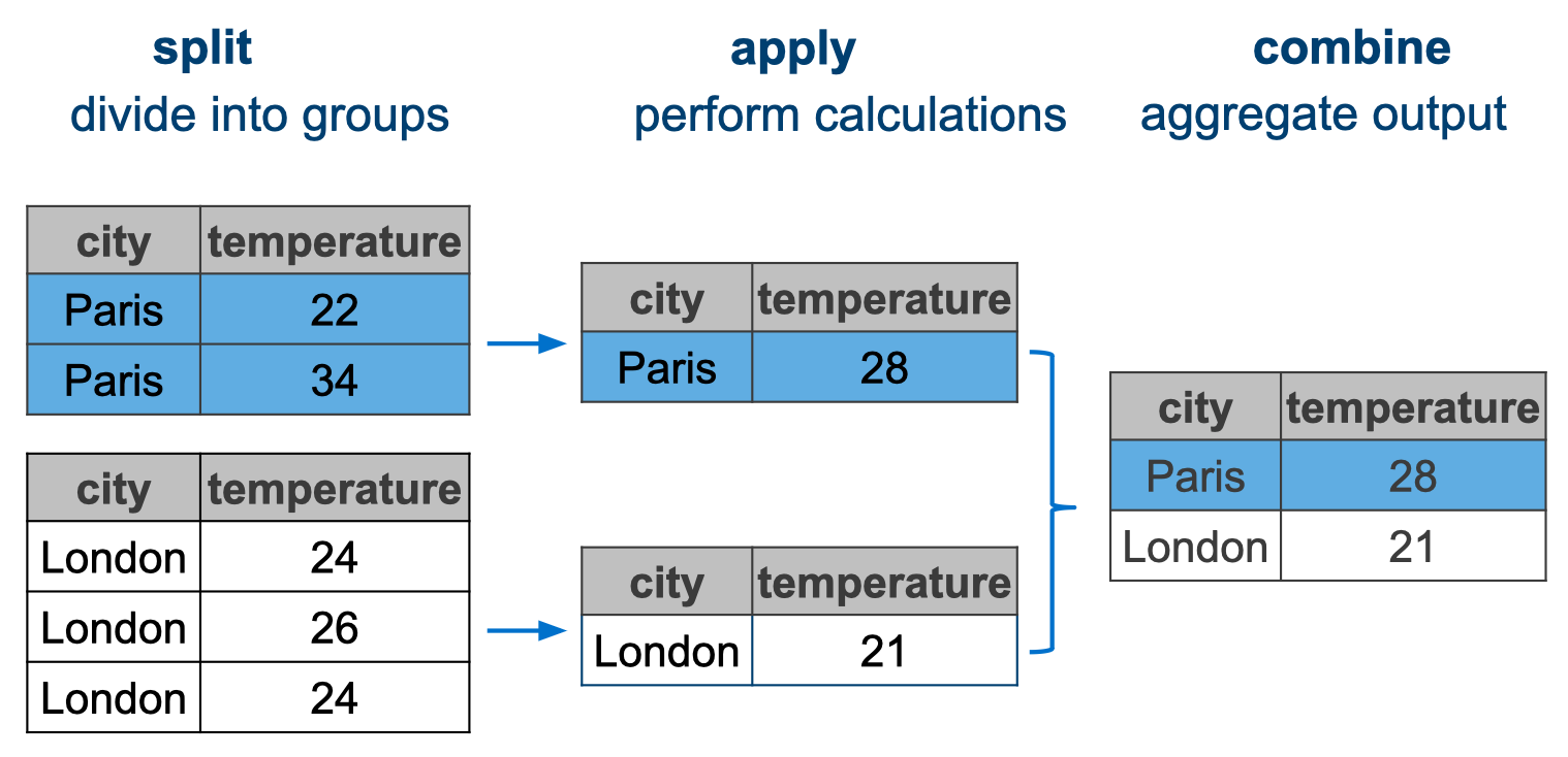
Conceptually, this kind of operation can be referred to as split-apply-combine, because we split the data, apply some function and then combine the outcome.
Let’s illustrate this with an example. Figure 11.1 shows a hypothetical data set, where we have temperature and rainfall measurements for different cities.
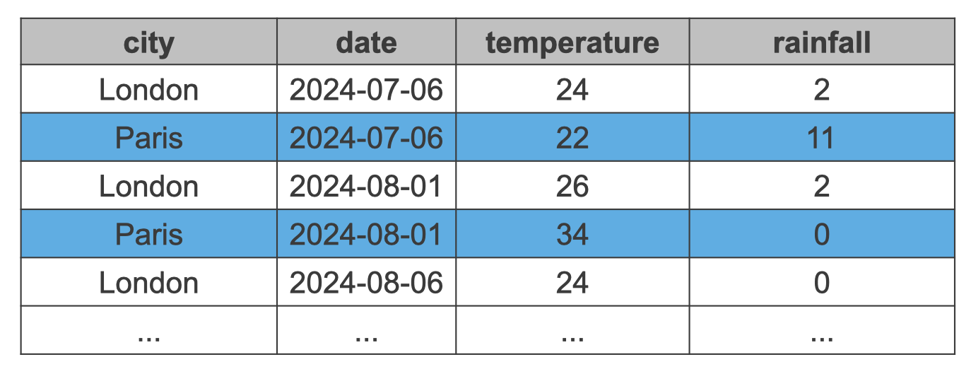
Let’s assume we were interested in the average temperature for each city. We would have to do the following:
- Split the data by
city - Calculate the average
temperature - Combine the outcome together in a new table
This is visualised in Figure 11.2.
11.4 Summary operations
Let’s put this into practice with our data set.
11.4.1 Summarising data
A common task in data analysis is to summarise variables to get the mean and the variation around it.
For example, let’s calculate what the mean and standard deviation are for weight.
We can achieve this task using the summarise() function.
surveys |>
  summarise(weight_mean = mean(weight, na.rm  = TRUE),
            weight_sd = sd(weight, na.rm = TRUE))
# A tibble: 1 × 2
weight_mean weight_sd
<dbl> <dbl>
1 42.7 36.6A couple of things to notice:
The output of summarise is a new table, where each column is named according to the input to summarise().
Within summarise() we should use functions for which the output is a single value. Also notice that, above, we used the na.rm option within the summary functions, so that they ignored missing values when calculating the respective statistics.
For these kind of summary statistics we can use .agg() - the aggregate function in pandas. You can apply this to a DataFrame or Series. It works on standard summary functions, listed below.
surveys["weight"].agg(
    weight_mean = "mean",
    weight_sd = "std"
)
weight_mean 42.672428
weight_sd 36.631259
Name: weight, dtype: float64
TipSummary functions
There are many functions whose input is a vector (or a column in a table) and the output is a single number. Here are several common ones:
| R | Example | Description |
|---|---|---|
mean |
mean(x, na.rm = TRUE) |
Arithmetic mean |
median |
median(x, na.rm = TRUE) |
Median |
sd |
sd(x, na.rm = TRUE) |
Standard deviation |
var |
var(x, na.rm = TRUE) |
Variance |
mad |
mad(x, na.rm = TRUE) |
Median absolute deviation |
min |
min(x, na.rm = TRUE) |
Minimum value |
max |
max(x, na.rm = TRUE) |
Maximum value |
sum |
sum(x, na.rm = TRUE) |
Sum of all values |
n_distinct |
n_distinct(x) |
Number of distinct (unique) values |
All of these have the option na.rm, which tells the function remove missing values before doing the calculation.
Python (pandas) |
Example (in .agg()) |
Description |
|---|---|---|
"mean" |
df["x"].agg("mean") |
Arithmetic mean |
"median" |
df["x"].agg("median") |
Median |
"std" |
df["x"].agg("std") |
Standard deviation |
"var" |
df["x"].agg("var") |
Variance |
"mad" |
df["x"].agg("mad") |
Mean absolute deviation |
"min" |
df["x"].agg("min") |
Minimum value |
"max" |
df["x"].agg("max") |
Maximum value |
"sum" |
df["x"].agg("sum") |
Sum of all values |
"nunique" |
df["x"].agg("nunique") |
Number of distinct (unique) values |
11.4.2 Grouped summaries
In most cases we want to calculate summary statistics across groups of our data.
We can achieve this by combining summarise() with the group_by() function. For example, let’s modify the previous example to calculate the summary for each sex group:
surveys |>
  group_by(sex) |>
  summarise(weight_mean = mean(weight, na.rm  = TRUE),
            weight_sd = sd(weight, na.rm = TRUE))
# A tibble: 3 × 3
sex weight_mean weight_sd
<chr> <dbl> <dbl>
1 F 42.2 36.8
2 M 43.0 36.2
3 <NA> 64.7 62.2The table output now includes both the columns we defined within summarise() as well as the grouping columns defined within group_by().
surveys.groupby("sex")["weight"].agg(
    weight_mean = "mean",
    weight_sd = "std"
).reset_index()
sex weight_mean weight_sd
0 F 42.170555 36.847958
1 M 42.995379 36.18498111.5 Counting data
Counting or tallying data is an extremely useful way of getting to know your data better.
11.5.1 Simple counting
We can use the count() function from dplyr to count data. It always returns the number of rows it counts.
For example, this gives us the total number of observations (rows) in our data set:
count(surveys)# A tibble: 1 × 1
n
<int>
1 35549We can use the .shape attribute. In pandas, each DataFrame has a .shape attribute that returns a tuple in the format (rows, columns).
So, .shape[0] will return the number of rows, whereas .shape[1] returns the number of columns.
For our surveys DataFrame we then get the number of rows by:
surveys.shape[0]35549We can also use that in combination with a conditional statement. For example, if we’re interested in all the observations from the year 1982.
# count the observations from the year 1982
surveys |>
  filter(year == 1982) |>
  count()
# A tibble: 1 × 1
n
<int>
1 1978surveys[surveys["year"] == 1982].shape[0]1978Or, slightly easier to read, with the .query() function:
surveys.query("year == 1982").shape[0]197811.5.2 Counting by group
Counting really comes into its own when we’re combining this with some grouping. For example, we might be interested in the number of observations for each year.
surveys |>
  count(year)
# A tibble: 26 × 2
year n
<dbl> <int>
1 1977 503
2 1978 1048
3 1979 719
4 1980 1415
5 1981 1472
6 1982 1978
7 1983 1673
8 1984 981
9 1985 1438
10 1986 942
# ℹ 16 more rowsWe can also easily visualise this (we can pipe straight into ggplot()). We use geom_col() to create a bar chart of the number of observations per year. We count by sex and use this variable to fill the colour of the bars.
surveys |>
  count(sex, year) |>
  ggplot(aes(x = year, y = n, fill = sex)) +
  geom_col()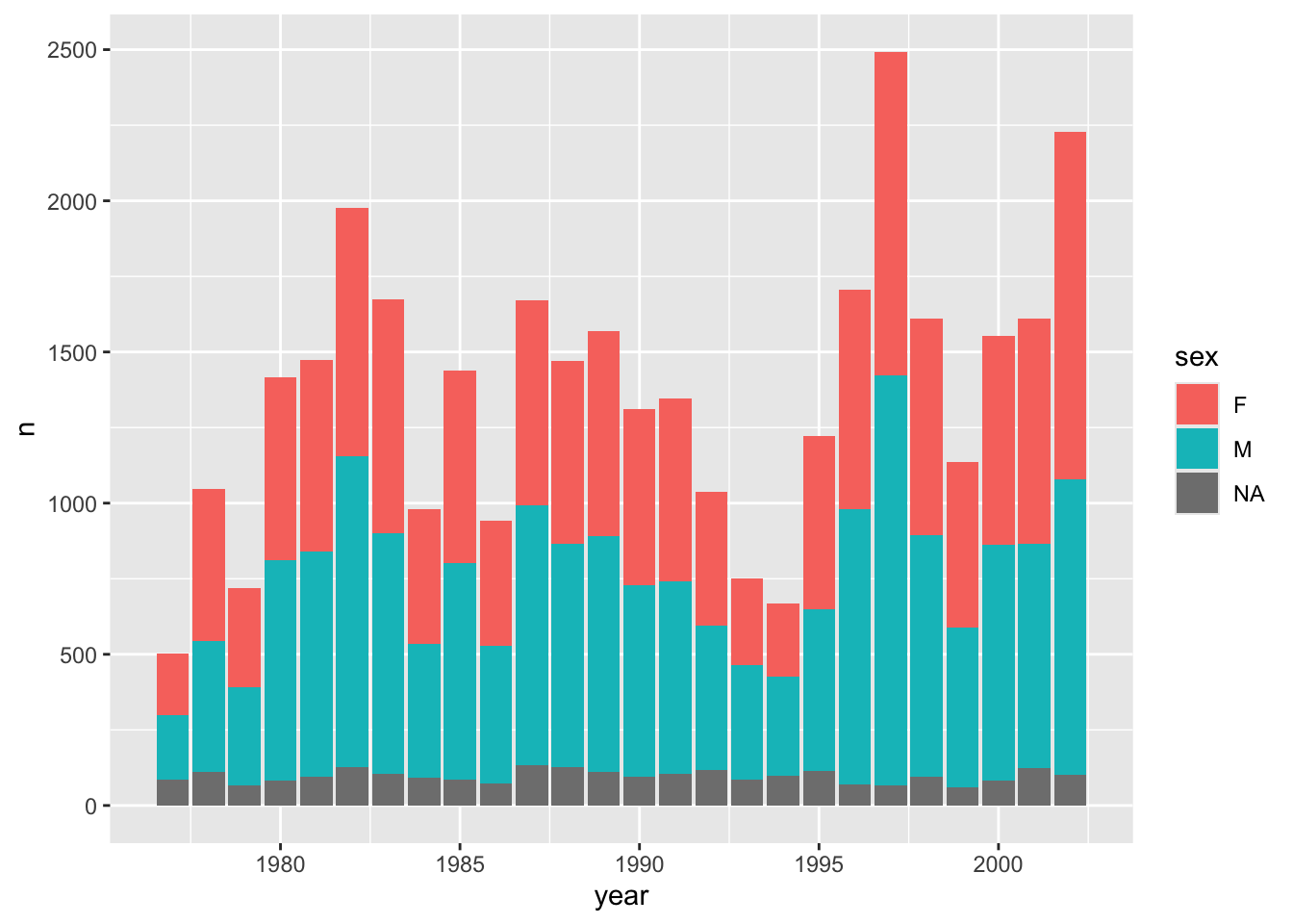
sex.
# Count number of rows for each year
counts = surveys.groupby("year").size().reset_index(name = "n")

# Look at the first few rows
counts.head()
year n
0 1977 503
1 1978 1048
2 1979 719
3 1980 1415
4 1981 1472Let’s expand this example a bit, where we count by two variables: sex and year. We then also plot the results, just to illustrate how useful that can be.
# Count observations by sex and year
counts = surveys.groupby(["sex", "year"]).size().reset_index(name = "n")
p = (ggplot(counts, aes(x = "year", y = "n", fill = "sex")) +
geom_col())
p.show()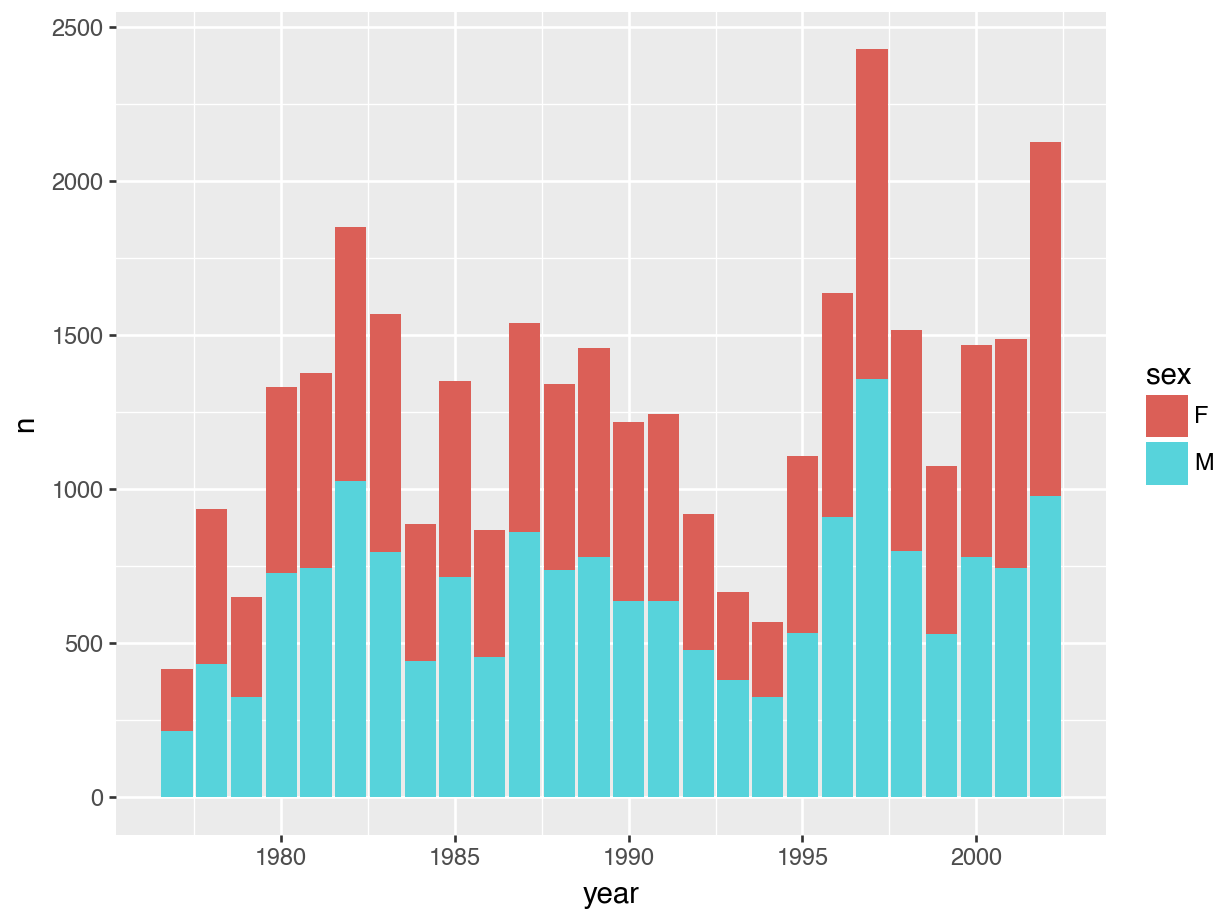
sex.
NoteSeaborn equivalent
This is not an exact equivalent to the plot above, because sns.barplot() gives dodged (side-by-side) groupings by default.
There is no native stacked bars in Seaborn, so you’d have to use the underlying matplotlib. We’re not covering this here, but feel free to search or use ChatGPT.
sns.barplot(
    data = counts,
    x = "year",
    y = "n",
    hue = "sex"   # fill = sex in ggplot
)

plt.title("Counts by year and sex")
plt.show()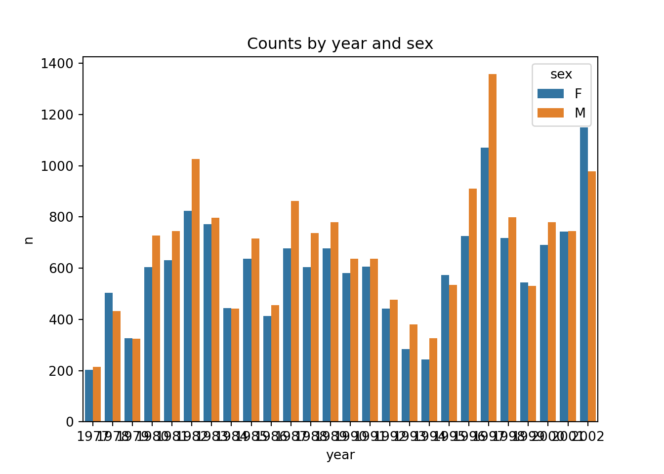
sex.
ImportantCounting within a summary pipeline
Often we want to do counting when we’re creating summaries. Let’s illustrate this with an example where we take the observations from 1981 and 1982, then calculate the mean weight and count the number of observations.
The count() function can’t be used within summarise(), but there is a special helper function called n(). Look at the following example, where we group by year, filter the data, create some summary statistic and also count the number of rows within each group.
surveys |>
  group_by(year) |>                                   # group the data
  filter(year %in% c(1981, 1982)) |>                  # filter a subset of years
  summarise(mean_weight = mean(weight, na.rm = TRUE), # calculate mean weight
            n_obs = n()) |>                           # number of rows
  ungroup()                                           # drop the grouping
# A tibble: 2 × 3
year mean_weight n_obs
<dbl> <dbl> <int>
1 1981 65.8 1472
2 1982 53.8 1978We need to do this in two steps:
- Filter out the relevant data
- Calculate the summary statistics
Here we’re using ( ) around the pipeline, so we can break up the code into different lines. This aids with readability, but doesn’t change how the code works!
# Group by year and summarise
summary = (
     surveys
    .query("year in [1981, 1982]")         # filter data based on year
    .groupby("year")                       # group by year
    .agg(                                  # create summary statistics
        mean_weight = ("weight", "mean"),  # calculate mean weights
        n_obs = ("weight", "count")        # count of non-NaN weights
    )
    .reset_index()                         # converts index into regular column
)

print(summary)
year mean_weight n_obs
0 1981 65.843888 1358
1 1982 53.765888 184111.5.3 Counting missing data
Oh, missing data! How we’ve missed you. For something that isn’t there, is has quite the presence. But, it is an important consideration in data analysis. We’ve already seen how we can remove missing data from and also explored ways to visualise them.
We have seen how to use the summary() function to find missing values. Here we’ll see (even more) ways to tally them.
We can use the is.na() function to great effect, within a summarise() pipeline. We can negate with !is.na() to find non-missing values. Again, using the sum() function then enables us to tally how many missing / non-missing values there are.
surveys |>
  summarise(obs_present = sum(!is.na(species_id)),    # count non-missing data
            obs_absent = sum(is.na(species_id)),      # count missing data
            n_obs = n(),                              # total number of rows
            percentage_absent =
              (obs_absent / n_obs) * 100) |>          # percentage of missing data
  ungroup()
# A tibble: 1 × 4
obs_present obs_absent n_obs percentage_absent
<int> <int> <int> <dbl>
1 34786 763 35549 2.15We can use the .isna() and .notna() functions to great effect. Again, we’re using the .sum() function to tally the numbers.
summary = pd.DataFrame([{
    "obs_present": surveys["species_id"].notna().sum(),
    "obs_absent": surveys["species_id"].isna().sum(),
    "n_obs": len(surveys),
    "percentage_absent": surveys["species_id"].isna().mean() * 100
}])

print(summary)
obs_present obs_absent n_obs percentage_absent
0 34786 763 35549 2.14633311.6 Grouped operations
11.6.1 Grouped filters
Sometimes it can be really handy to filter data, by group. In our surveys data, for example, you might be interested to find out what the minimum weight value is for each year. We can do that as follows:
surveys |>
  group_by(year) |>
  filter(weight == min(weight, na.rm = TRUE)) |>
  ungroup()
# A tibble: 94 × 9
record_id month day year plot_id species_id sex hindfoot_length weight
<dbl> <dbl> <dbl> <dbl> <dbl> <chr> <chr> <dbl> <dbl>
1 218 9 13 1977 1 PF M 13 4
2 1161 8 5 1978 6 PF F 16 6
3 1230 9 3 1978 19 PF M 16 6
4 1265 9 4 1978 15 PF F 16 6
5 1282 9 4 1978 4 PF F 16 6
6 1343 10 7 1978 11 PF F 15 6
7 1351 10 8 1978 2 PF M 15 6
8 1380 10 8 1978 3 PF F 16 6
9 1400 11 4 1978 19 PF M 15 6
10 1427 11 4 1978 21 PF F 15 6
# ℹ 84 more rowsYou can see that this outputs the minimum value, but if there are multiple entries for each year (such as in 1978), multiple rows returned. If we only wanted to get a single row per minimum value, per year, then we can use slice(1). This slices the first row of each group:
surveys |>
  group_by(year) |>
  filter(weight == min(weight, na.rm = TRUE)) |>
  slice(1) |>
  ungroup()
# A tibble: 26 × 9
record_id month day year plot_id species_id sex hindfoot_length weight
<dbl> <dbl> <dbl> <dbl> <dbl> <chr> <chr> <dbl> <dbl>
1 218 9 13 1977 1 PF M 13 4
2 1161 8 5 1978 6 PF F 16 6
3 1923 7 25 1979 18 PF F NA 6
4 2506 2 25 1980 3 PF F 15 5
5 4052 4 5 1981 3 PF F 15 4
6 5346 2 22 1982 21 PF F 14 4
7 8736 12 8 1983 19 RM M 17 4
8 8809 2 4 1984 16 RM F 14 7
9 9790 1 19 1985 16 RM F 16 4
10 11299 3 9 1986 3 RM F 16 7
# ℹ 16 more rowsfirst_min_per_year = (
surveys.dropna(subset=["weight"]) # 1. remove rows with missing weight
.groupby("year", group_keys = False) # 2. split data into groups by year
.apply(lambda g: g.loc[g["weight"].idxmin()]) # 3. in each group, pick row with min weight
.reset_index(drop = True) # 4. clean up index
)
first_min_per_year.head() record_id month day year plot_id species_id sex hindfoot_length weight
0 218 9 13 1977 1 PF M 13.0 4.0
1 1161 8 5 1978 6 PF F 16.0 6.0
2 1923 7 25 1979 18 PF F NaN 6.0
3 2506 2 25 1980 3 PF F 15.0 5.0
4 4052 4 5 1981 3 PF F 15.0 4.0Here we’re adding group_keys = False to the groupby() function, so we’re not adding the group labels to the index. We are using .idxmin() to find the minimum index id.
11.6.2 Grouped changes
Sometimes you might need to add a new variable to our table, based on different groups. Let’s say we want to see how many female and male observations there are in our surveys data set for each year.
We’re also interested in the percentage of female observations out of the total number of observations where sex was recorded.
We have the following number of female / male observations:
surveys |>
  group_by(year) |>
  summarise(n_obs_f = sum(sex == "F", na.rm = TRUE),
            n_obs_m = sum(sex == "M", na.rm = TRUE)) |>
  ungroup()
# A tibble: 26 × 3
year n_obs_f n_obs_m
<dbl> <int> <int>
1 1977 204 214
2 1978 503 433
3 1979 327 324
4 1980 605 727
5 1981 631 745
6 1982 823 1027
7 1983 771 797
8 1984 445 443
9 1985 636 716
10 1986 414 455
# ℹ 16 more rowsNow, let’s say we’d be interested in the percentage of female observations out of the total of observations where it was scored. We’d have to add a new column. Adding new columns is, as we’ve seen before, a job for mutate().
surveys |>
  group_by(year) |>
  summarise(n_obs_f = sum(sex == "F", na.rm = TRUE),
            n_obs_m = sum(sex == "M", na.rm = TRUE)) |>
  ungroup() |>
  mutate(female_pct = n_obs_f / (n_obs_f + n_obs_m) * 100)
# A tibble: 26 × 4
year n_obs_f n_obs_m female_pct
<dbl> <int> <int> <dbl>
1 1977 204 214 48.8
2 1978 503 433 53.7
3 1979 327 324 50.2
4 1980 605 727 45.4
5 1981 631 745 45.9
6 1982 823 1027 44.5
7 1983 771 797 49.2
8 1984 445 443 50.1
9 1985 636 716 47.0
10 1986 414 455 47.6
# ℹ 16 more rowsThe nice thing about chaining all these commands is that we can quickly build up what we want. We could, for example, easily plot the outcome of this.
surveys |>
  group_by(year) |>
  summarise(n_obs_f = sum(sex == "F", na.rm = TRUE),
            n_obs_m = sum(sex == "M", na.rm = TRUE)) |>
  ungroup() |>
  mutate(female_pct = n_obs_f / (n_obs_f + n_obs_m) * 100) |>
  ggplot(aes(x = year, y = female_pct)) +
  geom_line()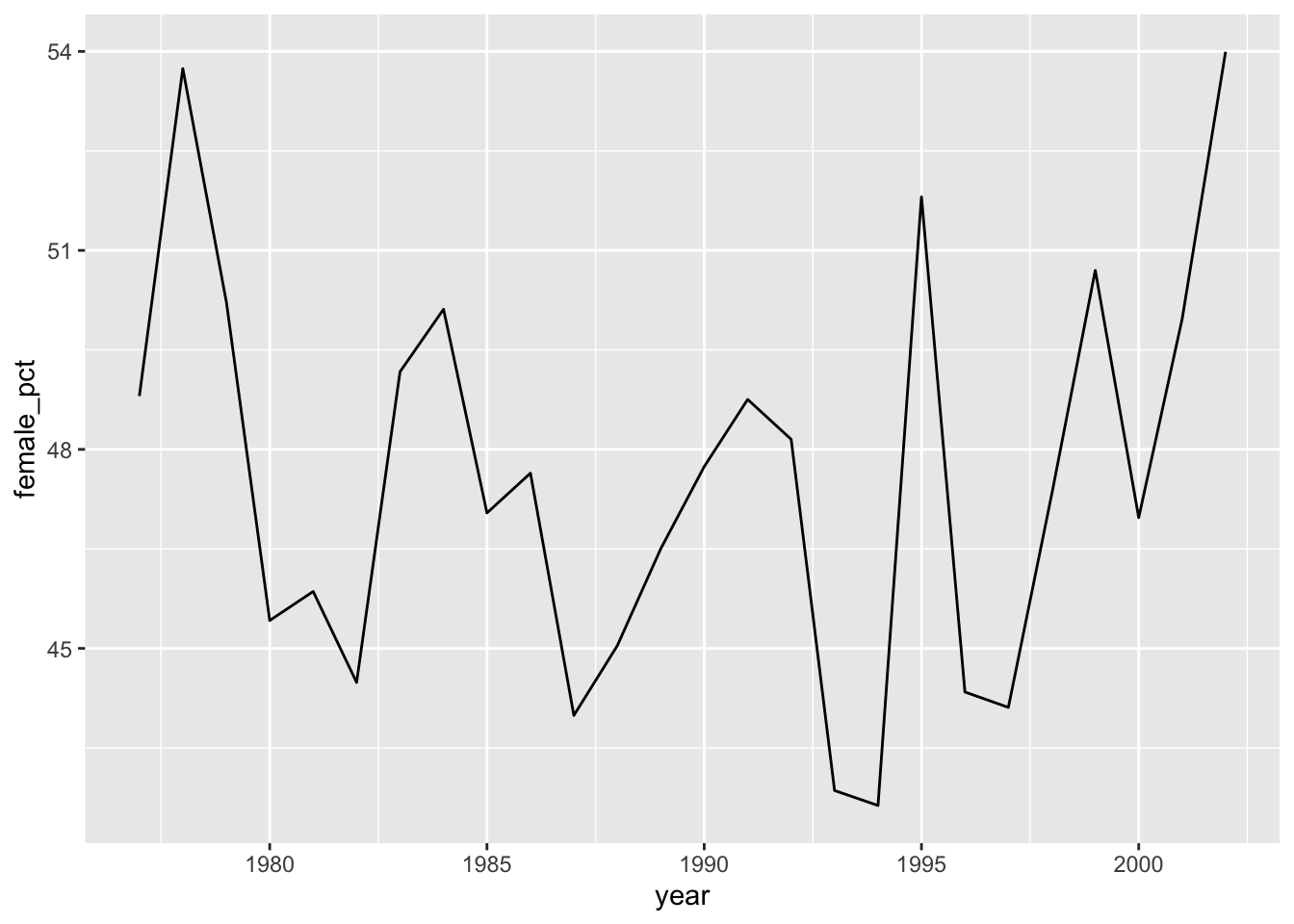
summary = (
    surveys
    .groupby("year")
    .agg(n_obs_f = ("sex", lambda x: (x == "F").sum()),
         n_obs_m = ("sex", lambda x: (x == "M").sum()))
    .reset_index()
)

summary.head()
year n_obs_f n_obs_m
0 1977 204 214
1 1978 503 433
2 1979 327 324
3 1980 605 727
4 1981 631 745# Add female percentage column
summary["female_pct"] = summary["n_obs_f"] / (summary["n_obs_f"] + summary["n_obs_m"]) * 100
summary.head() year n_obs_f n_obs_m female_pct
0 1977 204 214 48.803828
1 1978 503 433 53.739316
2 1979 327 324 50.230415
3 1980 605 727 45.420420
4 1981 631 745 45.857558Now we have the table, we can easily plot it to get a better sense of any trends.
p = (ggplot(summary, aes(x = "year", y = "female_pct")) +
    geom_line())

p.show()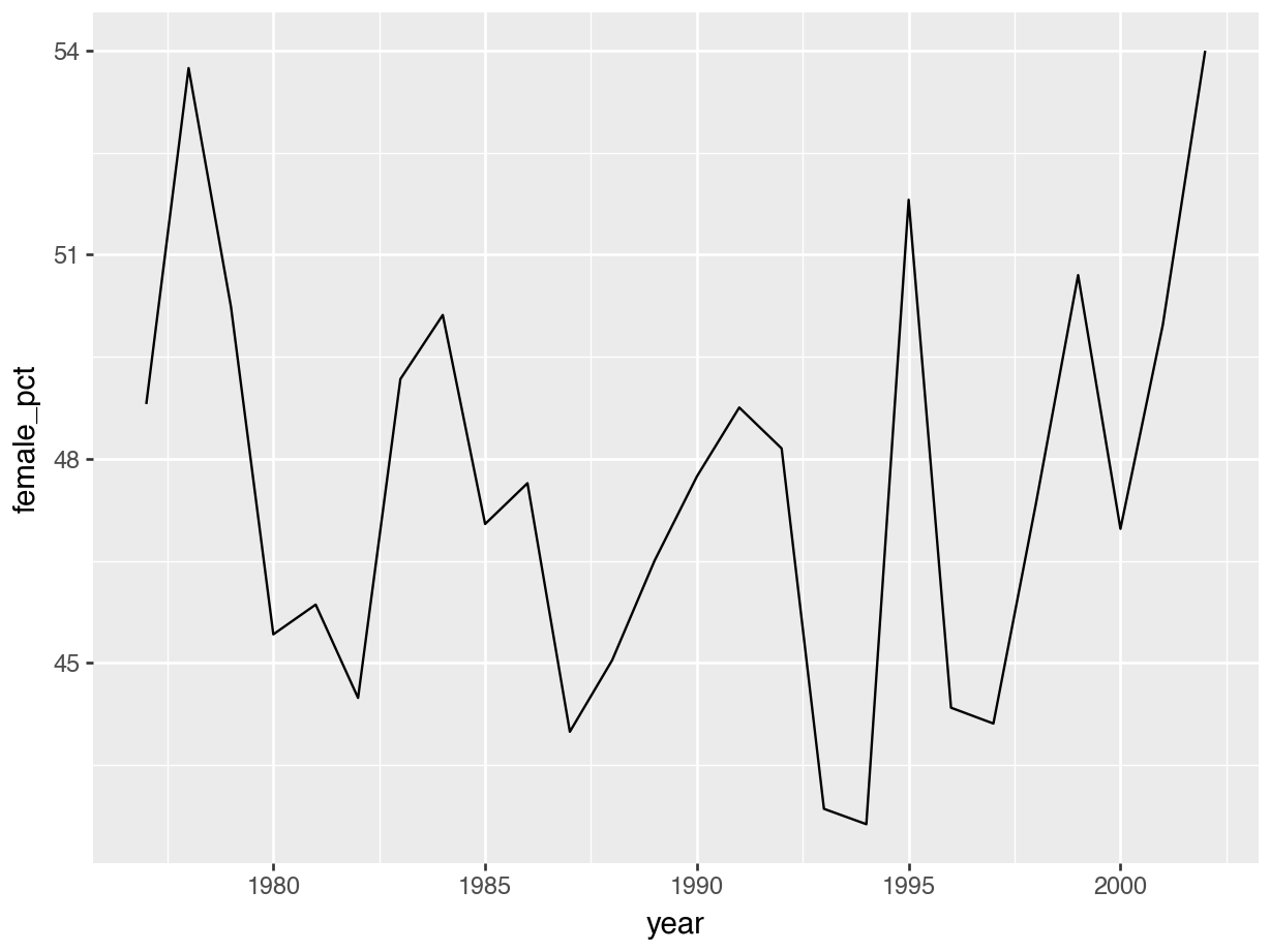
NoteSeaborn equivalent
# seaborn lineplot
sns.lineplot(
    data = summary,
    x = "year",
    y = "female_pct"
)

plt.title("Female percentage by year")
plt.show()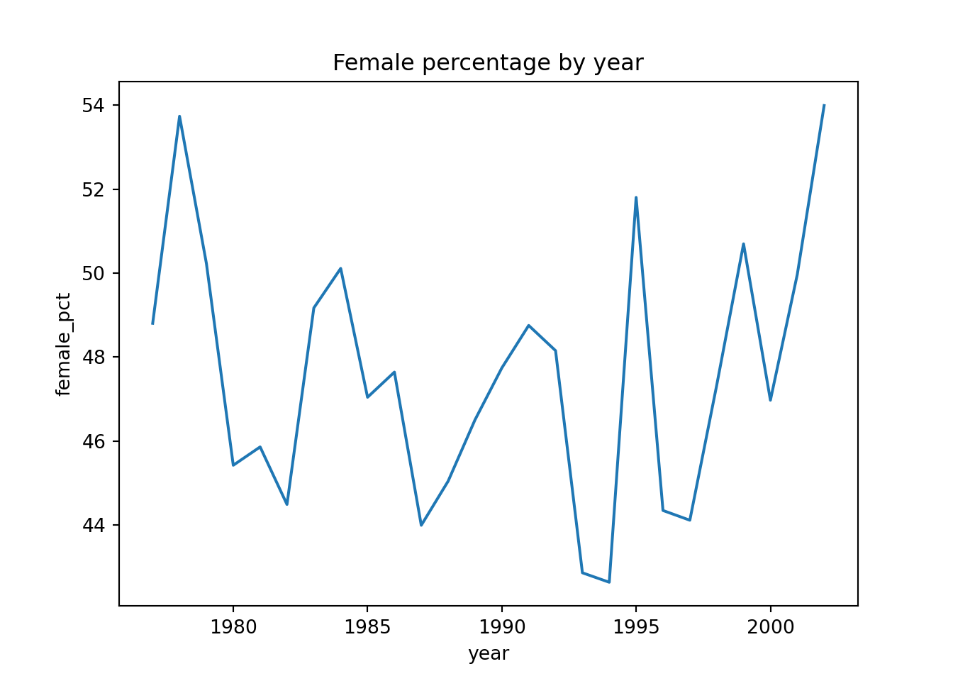
WarningTo ungroup or not ungroup (R-only)
Each time you do a grouped operation, it’s good practice to remove the grouping afterwards. If you don’t, then you might unintentionally be doing operations within the groups later on.
Let’s illustrate this with an example. We’ll take out any missing values, to simplify things.
obs_count <- surveys |>
  drop_na() |>
  group_by(sex, year) |>
  summarise(n_obs = n())
`summarise()` has grouped output by 'sex'. You can override using the `.groups`
argument.obs_count# A tibble: 52 × 3
# Groups: sex [2]
sex year n_obs
<chr> <dbl> <int>
1 F 1977 123
2 F 1978 430
3 F 1979 297
4 F 1980 442
5 F 1981 482
6 F 1982 672
7 F 1983 758
8 F 1984 436
9 F 1985 624
10 F 1986 400
# ℹ 42 more rowsLet’s say we now wanted to transform the n_obs variable to a percentage of the total number of observations in the entire data set (which is 30676).
obs_count <- obs_count |>
  mutate(n_obs_pct = n_obs / sum(n_obs) * 100)
We’d expect these values in n_obs_pct to add up to 100%.
sum(obs_count$n_obs_pct)[1] 200However, they add up to 200 instead! Why? That’s because the table was still grouped by sex and as such, the percentages were calculated by each sex group. There are two of them (F, M - we filtered out the missing values), so the percentages add up to 100% within each sex group.
The way to avoid this issue is to ensure we remove any groups from our table, which we can do with ungroup(). Here’s the full string of commands, with the ungrouping step added:
obs_count <- surveys |>
  drop_na() |>                                  # remove all NAs
  group_by(sex, year) |>                        # group by sex, year
  summarise(n_obs = n()) |>                     # get number of rows
  ungroup() |>                                  # ungroup here
  mutate(n_obs_pct = n_obs / sum(n_obs) * 100)  # calculate percentage
`summarise()` has grouped output by 'sex'. You can override using the `.groups`
argument.We can check the percentages again and see that all is well:
sum(obs_count$n_obs_pct)[1] 100In pandas, grouping only affects the aggregation step. Once you run .groupby().agg() or .groupby().sum(), the grouping is gone — the resulting DataFrame is no longer grouped.
So, things are easier in Python in this respect. Sometimes it’s nice to be smug.
11.7 Exercises
11.7.1 Grouped summaries: infections
11.7.2 Grouped operations: infections
ExerciseExercise 2 - Grouped operations
Level:
We’ll keep using the infections data set.
To add a bit of fun, we’ll combine the filtering with making some changes to our data and plotting these. These are the kind of operations you’ll be doing a lot when exploring and analysis your data, so it’s good to practise!
Have a look at the plot below and try to recreate it as accurately as possible:

AnswerAnswer
We’ll assume you still have the data loaded.
infections |>
  filter(!is.na(hospital)) |>
  group_by(hospital) |>
  arrange(desc(crp_level)) |>
  slice(1:10) |>
  summarise(mean_crp = mean(crp_level, na.rm = TRUE),
            log_crp = log(mean_crp)) |>
  ungroup() |>
  ggplot(aes(x = hospital, y = log_crp)) +
  geom_point() +
  geom_segment(aes(x = hospital, xend = hospital, y = 3.8, yend = log_crp)) +
  labs(title = "Average log values for CRP",
       subtitle = "calculated on top 10 highest values within each hospital",
       x = "",
       y = "CRP level (log values)")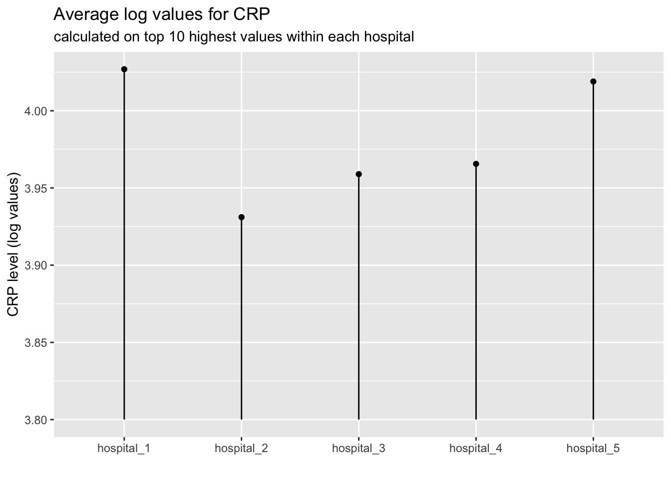
import numpy as np

infections_result = (
    infections
    .dropna(subset=["hospital"])
    .sort_values("crp_level", ascending = False)        # arrange data
    .groupby("hospital", as_index = False)              # group data
    .head(10)                                           # get first 10 rows
    .groupby("hospital", as_index = False)              # group again
    .agg(mean_crp = ("crp_level", "mean"))              # mean values
    .assign(log_crp = lambda d: np.log(d["mean_crp"]))  # calculate log
)
p = (
ggplot(infections_result, aes(x = "hospital", y = "log_crp")) +
geom_point() +
geom_segment(aes(x = "hospital", xend = "hospital", y = 3.8, yend = "log_crp")) +
labs(
title = "Average log values for CRP",
subtitle = "calculated on top 10 highest values within each hospital",
x = "",
y = "CRP level (log values)"
)
)
p.show()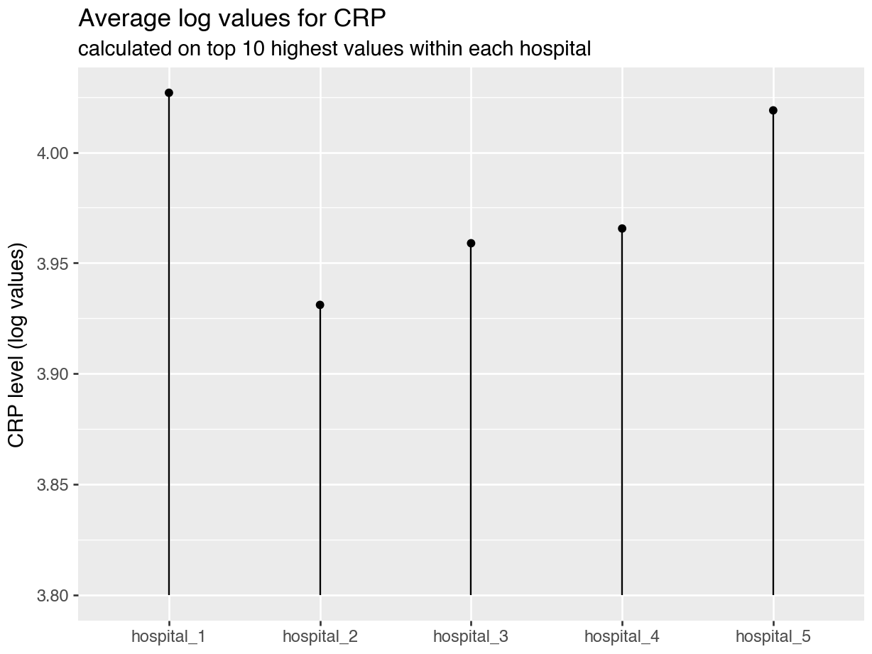
11.8 Summary
TipKey points
- We can split our data into groups and apply operations to each group.
- We can then combine the outcomes in a new table.
- We use
summarise()to calculate summary statistics (e.g. mean, median, maximum, etc). - Using pipes with groups (e.g.
group_by() |> summarise()) we can calculate those summaries across groups. - We can also filter (
group_by() |> filter()) or create new columns (group_by() |> mutate()). - It is good practice to remove grouping (with
ungroup()) from tables aftergroup_by()operations, to avoid issues with retained groupings.
- We can split our data into groups and apply operations to each group.
- We can then combine the outcomes in a new table.
- We use
.agg()to calculate summary statistics (e.g. mean, median, maximum, etc). - We can use
.groupby()to group by variables in our data. - Using grouped filters we can find values for each group within our data.