# install if needed
install.packages("visdat")10 Manipulating rows
TipLearning objectives
- Learn to order and arrange rows.
- Be able to find and retain unique rows.
- Understand how logical operators are used.
- Implement conditional statements to filter specific data.
- Be able to identify and decide how to deal with missing data.
10.1 Context
Data sets can contain large quantities of observations. Often we are only interested in part of the data at a given time. We can deal with this by manipulating rows.
10.2 Section setup
We’ll continue this section with the script named 03_session. If needed, add the following code to the top of your script and run it.
In this section we will use a new package, called visdat, to visualise where we have missing data. Install it as follows:
# A collection of R packages designed for data science
library(tidyverse)

# Package to visualise missing data
library(visdat)

surveys <- read_csv("data/surveys.csv")
We’ll continue this section with the Notebook named 03_session. Add the following code to the first cell and run it.
We’ll use a new package, so install if needed from the terminal:
mamba install conda-forge::missingnoThen, if needed, add the following code to the top of your script and run it.
# A Python data analysis and manipulation tool
import pandas as pd
import numpy as np

# Python equivalent of `ggplot2`
from plotnine import *

# If using seaborn for plotting
import seaborn as sns
import matplotlib.pyplot as plt

# Load missingno
import missingno as msno

surveys = pd.read_csv("data/surveys.csv")
10.3 Arranging data
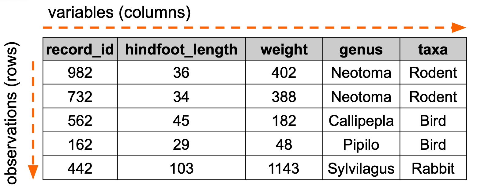
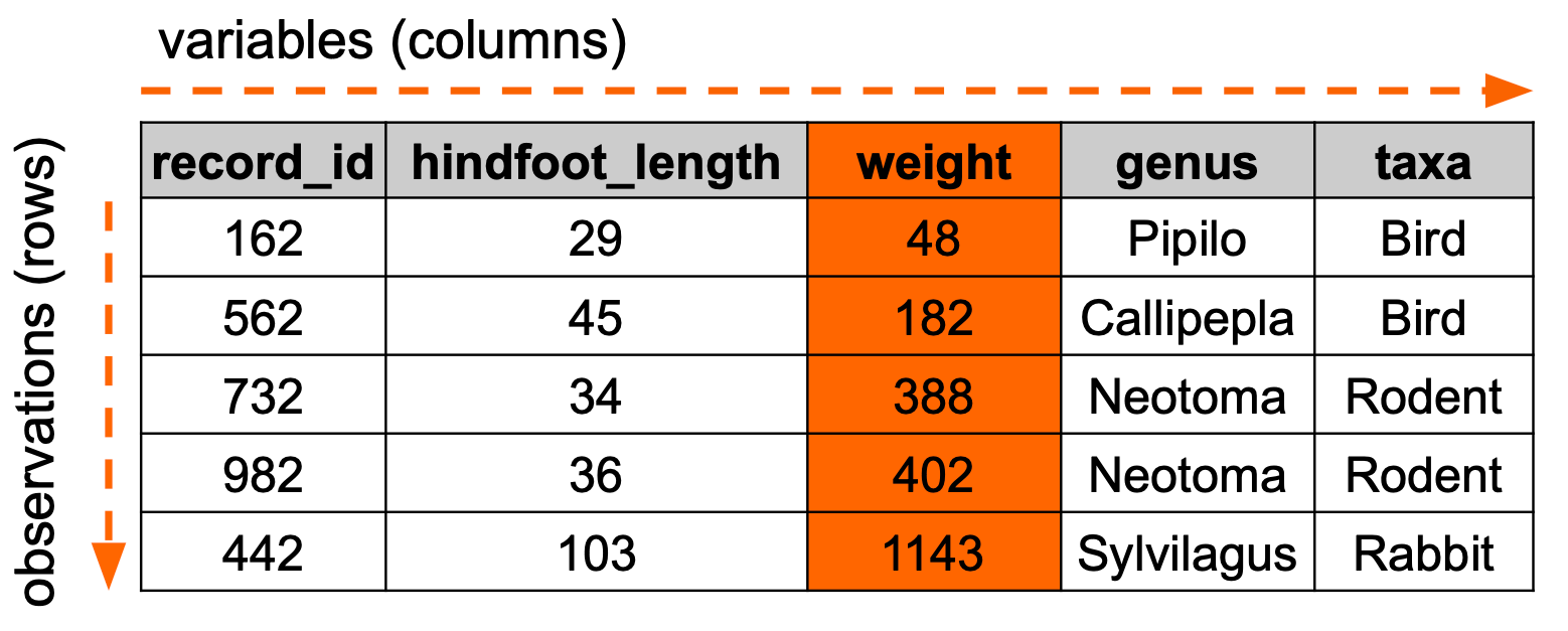
We often want to order data in a certain way, for example ordering by date or in alphabetically. The example below illustrates how we would order data based on weight:
Let’s illustrate this with the surveys data set, arranging the data based on year.
surveys |>
  arrange(year)
# A tibble: 35,549 × 9
record_id month day year plot_id species_id sex hindfoot_length weight
<dbl> <dbl> <dbl> <dbl> <dbl> <chr> <chr> <dbl> <dbl>
1 1 7 16 1977 2 NL M 32 NA
2 2 7 16 1977 3 NL M 33 NA
3 3 7 16 1977 2 DM F 37 NA
4 4 7 16 1977 7 DM M 36 NA
5 5 7 16 1977 3 DM M 35 NA
6 6 7 16 1977 1 PF M 14 NA
7 7 7 16 1977 2 PE F NA NA
8 8 7 16 1977 1 DM M 37 NA
9 9 7 16 1977 1 DM F 34 NA
10 10 7 16 1977 6 PF F 20 NA
# ℹ 35,539 more rowsIf we’d want to arrange the data in descending order (most recent to oldest), we would employ the desc() helper function:
surveys |>
  arrange(desc(year))
# A tibble: 35,549 × 9
record_id month day year plot_id species_id sex hindfoot_length weight
<dbl> <dbl> <dbl> <dbl> <dbl> <chr> <chr> <dbl> <dbl>
1 33321 1 12 2002 1 DM M 38 44
2 33322 1 12 2002 1 DO M 37 58
3 33323 1 12 2002 1 PB M 28 45
4 33324 1 12 2002 1 AB <NA> NA NA
5 33325 1 12 2002 1 DO M 35 29
6 33326 1 12 2002 2 OT F 20 26
7 33327 1 12 2002 2 OT M 20 24
8 33328 1 12 2002 2 OT F 21 22
9 33329 1 12 2002 2 DM M 37 47
10 33330 1 12 2002 2 DO M 35 51
# ℹ 35,539 more rowsWe can read that bit of code as “take the surveys data set, send it to the arrange() function and ask it to arrange the data in descending order (using desc()) based on the year column”.
We can also combine this approach with multiple variables, for example arranging data based on descending year and (ascending) hindfoot length:
surveys |>
  arrange(desc(year), hindfoot_length)
# A tibble: 35,549 × 9
record_id month day year plot_id species_id sex hindfoot_length weight
<dbl> <dbl> <dbl> <dbl> <dbl> <chr> <chr> <dbl> <dbl>
1 33647 3 14 2002 3 PF M 9 8
2 35301 12 8 2002 4 PF M 13 6
3 35506 12 31 2002 6 PF M 13 8
4 34281 6 15 2002 23 RM F 14 9
5 34663 7 14 2002 16 RM M 14 7
6 35101 11 10 2002 9 PF M 14 7
7 35487 12 29 2002 23 RO F 14 13
8 33429 2 9 2002 3 PF M 15 8
9 33535 2 10 2002 13 PF F 15 7
10 33556 2 10 2002 5 RO M 15 9
# ℹ 35,539 more rows
TipShorthand for
desc()
We can also use a shorthand for desc(), by using preceding the variable with -:
surveys |>
  arrange(-year)
surveys.sort_values(by = "year") record_id month day year ... species_id sex hindfoot_length weight
0 1 7 16 1977 ... NL M 32.0 NaN
343 344 10 18 1977 ... NL NaN NaN NaN
342 343 10 18 1977 ... PF NaN NaN NaN
341 342 10 18 1977 ... DM M 34.0 25.0
340 341 10 18 1977 ... DS M 50.0 NaN
... ... ... ... ... ... ... ... ... ...
34063 34064 5 16 2002 ... PP F 23.0 18.0
34064 34065 5 16 2002 ... DO M 36.0 32.0
34065 34066 5 16 2002 ... DO M 37.0 29.0
34059 34060 5 16 2002 ... DM M 36.0 55.0
35548 35549 12 31 2002 ... NaN NaN NaN NaN
[35549 rows x 9 columns]If we’d want to arrange the data in descending order (most recent to oldest), we would specify this with the ascending = False argument:
surveys.sort_values(by = "year", ascending = False) record_id month day year ... species_id sex hindfoot_length weight
35548 35549 12 31 2002 ... NaN NaN NaN NaN
34060 34061 5 16 2002 ... PB M 27.0 37.0
34066 34067 5 16 2002 ... DM F 36.0 50.0
34065 34066 5 16 2002 ... DO M 37.0 29.0
34064 34065 5 16 2002 ... DO M 36.0 32.0
... ... ... ... ... ... ... ... ... ...
341 342 10 18 1977 ... DM M 34.0 25.0
342 343 10 18 1977 ... PF NaN NaN NaN
343 344 10 18 1977 ... NL NaN NaN NaN
344 345 11 12 1977 ... DM F 34.0 45.0
0 1 7 16 1977 ... NL M 32.0 NaN
[35549 rows x 9 columns]We can also combine this approach with multiple variables, for example arranging data based on descending year and (ascending) hindfoot length:
surveys.sort_values(
    by = ["year", "hindfoot_length"],
    ascending = [False, True]
)
record_id month day year ... species_id sex hindfoot_length weight
33646 33647 3 14 2002 ... PF M 9.0 8.0
35300 35301 12 8 2002 ... PF M 13.0 6.0
35505 35506 12 31 2002 ... PF M 13.0 8.0
34280 34281 6 15 2002 ... RM F 14.0 9.0
34662 34663 7 14 2002 ... RM M 14.0 7.0
... ... ... ... ... ... ... ... ... ...
494 495 12 11 1977 ... NL NaN NaN NaN
496 497 12 11 1977 ... OT NaN NaN NaN
499 500 12 11 1977 ... OT NaN NaN NaN
500 501 12 11 1977 ... OT NaN NaN NaN
502 503 12 11 1977 ... NaN NaN NaN NaN
[35549 rows x 9 columns]10.4 Finding unique values
Sometimes it is useful to retain rows with unique combinations of some of our variables (i.e. remove any duplicated rows). We often use this to get a quick view on what groups we have in the data.
Let’s say we wanted to see which groups we have within the sex column in our surveys data set.
This can be do this with the distinct() function.
surveys |>
  distinct(sex)
# A tibble: 3 × 1
sex
<chr>
1 M
2 F
3 <NA> We can do this by specifying which column we’d like to get the unique values from. We then use .drop_duplicates() to remove all the duplicate values:
surveys[["sex"]].drop_duplicates() sex
0 M
2 F
13 NaNWe can also combine this approach across multiple variables. For example, we could check which sex groups appear across which years. We simply add year to our original code.
surveys |>
  distinct(sex, year)
# A tibble: 78 × 2
sex year
<chr> <dbl>
1 M 1977
2 F 1977
3 <NA> 1977
4 <NA> 1978
5 M 1978
6 F 1978
7 F 1979
8 M 1979
9 <NA> 1979
10 M 1980
# ℹ 68 more rowssurveys[["sex", "year"]].drop_duplicates() sex year
0 M 1977
2 F 1977
13 NaN 1977
503 NaN 1978
504 M 1978
... ... ...
31711 M 2001
31748 NaN 2001
33320 M 2002
33323 NaN 2002
33325 F 2002
[78 rows x 2 columns]10.5 Filtering by condition
Often we want to filter our data based on specific conditions / properties in the data. For example, in our data set you might want to filter for certain years, a specific weight range or only get all the observations for the first 100 record IDs.
Before we delve into this, it is important to understand that when we set a condition like above, the output is a logical vector. Let’s illustrate this with a very basic example.
Assume we have a series of year values, stored in an object called some_years. If we’d be interested in all the values where the year is before 2000, we would do the following:
some_years <- c(1985, 1990, 1999, 1995, 2010, 2000)
some_years < 2000
[1] TRUE TRUE TRUE TRUE FALSE FALSEWhat is happening is that, for each value in some_years, the computer checks against the condition: is that value smaller than 2000? If it is, it returns TRUE. If not, it returns FALSE.
For this example we’ll keep using pandas, for consistency. Since we’re only dealing with a simple, one-dimensional bunch of data, we create a pandas Series:
some_years = pd.Series([1985, 1990, 1999, 1995, 2010, 2000])
result = some_years < 2000

result
0 True
1 True
2 True
3 True
4 False
5 False
dtype: boolWhat is happening is that, for each value in some_years, the computer checks against the condition: is that value smaller than 2000? If it is, it returns True. If not, it returns False.
We can expand on this and supply multiple conditions. We do this by using the logical operators & (AND) and | (OR). For example, if we wanted the years between 1990 and 2000:
# both conditions have to be true
some_years > 1990 & some_years < 2000
[1] FALSE FALSE TRUE TRUE FALSE FALSEAnd if we wanted the years below 1990 or above 2000, then:
# only one or the other of the conditions has to be true
some_years < 1990 | some_years > 2000
[1] TRUE FALSE FALSE FALSE TRUE FALSE# both conditions have to be true
result = (some_years > 1990) & (some_years < 2000)
result0 False
1 False
2 True
3 True
4 False
5 False
dtype: boolAnd if we wanted the years below 1990 or above 2000, then:
# only one or the other of the conditions has to be true
result = (some_years < 1990) | (some_years > 2000)

result
0 True
1 False
2 False
3 False
4 True
5 False
dtype: boolThis concept is also applied to tables. We could filter across all rows in the surveys data set, for a hindfoot_length of larger than 31 mm. Conceptually, the computer does what is displayed in the Figure 10.1.
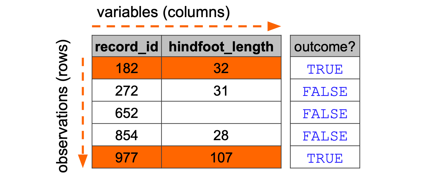
hindfoot_length > 31). If the outcome is TRUE then the row is returned.
We implement this as follows.
surveys |>
  filter(hindfoot_length > 31)
# A tibble: 15,729 × 9
record_id month day year plot_id species_id sex hindfoot_length weight
<dbl> <dbl> <dbl> <dbl> <dbl> <chr> <chr> <dbl> <dbl>
1 1 7 16 1977 2 NL M 32 NA
2 2 7 16 1977 3 NL M 33 NA
3 3 7 16 1977 2 DM F 37 NA
4 4 7 16 1977 7 DM M 36 NA
5 5 7 16 1977 3 DM M 35 NA
6 8 7 16 1977 1 DM M 37 NA
7 9 7 16 1977 1 DM F 34 NA
8 11 7 16 1977 5 DS F 53 NA
9 12 7 16 1977 7 DM M 38 NA
10 13 7 16 1977 3 DM M 35 NA
# ℹ 15,719 more rowssurveys[surveys["hindfoot_length"] > 31] record_id month day year ... species_id sex hindfoot_length weight
0 1 7 16 1977 ... NL M 32.0 NaN
1 2 7 16 1977 ... NL M 33.0 NaN
2 3 7 16 1977 ... DM F 37.0 NaN
3 4 7 16 1977 ... DM M 36.0 NaN
4 5 7 16 1977 ... DM M 35.0 NaN
... ... ... ... ... ... ... .. ... ...
35533 35534 12 31 2002 ... DM M 37.0 56.0
35534 35535 12 31 2002 ... DM M 37.0 53.0
35535 35536 12 31 2002 ... DM F 35.0 42.0
35536 35537 12 31 2002 ... DM F 36.0 46.0
35547 35548 12 31 2002 ... DO M 36.0 51.0
[15729 rows x 9 columns]Another option would be to use the .query() function. This is functionally equivalent, but a bit easier to read.
surveys.query("hindfoot_length > 31") record_id month day year ... species_id sex hindfoot_length weight
0 1 7 16 1977 ... NL M 32.0 NaN
1 2 7 16 1977 ... NL M 33.0 NaN
2 3 7 16 1977 ... DM F 37.0 NaN
3 4 7 16 1977 ... DM M 36.0 NaN
4 5 7 16 1977 ... DM M 35.0 NaN
... ... ... ... ... ... ... .. ... ...
35533 35534 12 31 2002 ... DM M 37.0 56.0
35534 35535 12 31 2002 ... DM M 37.0 53.0
35535 35536 12 31 2002 ... DM F 35.0 42.0
35536 35537 12 31 2002 ... DM F 36.0 46.0
35547 35548 12 31 2002 ... DO M 36.0 51.0
[15729 rows x 9 columns]This only keeps the observations where hindfoot_length > 31, in this case 15729 observations.
ImportantConditional operators
To set filtering conditions, use the following relational operators:
>is greater than>=is greater than or equal to<is less than<=is less than or equal to==is equal to!=is different from%in%is contained in
To combine conditions, use the following logical operators:
&AND|OR
Some functions return logical results and can be used in filtering operations:
is.na(x)returns TRUE if a value in x is missing
The ! can be used to negate a logical condition:
!is.na(x)returns TRUE if a value in x is NOT missing!(x %in% y)returns TRUE if a value in x is NOT present in y
To set filtering conditions, use the following relational operators:
>is greater than>=is greater than or equal to<is less than<=is less than or equal to==is equal to!=is different from.isin([...])is contained in
To combine conditions, use the following logical operators:
&AND|OR
Some functions return logical results and can be used in filtering operations:
df["x"].isna()returns True if a value in x is missing
The ~ (bitwise NOT) can be used to negate a logical condition:
~df["x"].isna()returns True if a value in x is NOT missing~df["x"].isin(["y"])returns True if a value in x is NOT present in"y"
10.6 Missing data revisited
It’s important to carefully consider how to deal with missing data, as we have previously seen. It’s easy enough to filter out all rows that contain missing data, however this is rarely the best course of action, because you might accidentally throw out useful data in columns that you’ll need later.
Furthermore, it’s often a good idea to see if there is any structure in your missing data. Maybe certain variables are consistently absent, which could tell you something about your data.
We could filter out all the missing weight values as follows:
surveys |>
  filter(!is.na(weight))
# A tibble: 32,283 × 9
record_id month day year plot_id species_id sex hindfoot_length weight
<dbl> <dbl> <dbl> <dbl> <dbl> <chr> <chr> <dbl> <dbl>
1 63 8 19 1977 3 DM M 35 40
2 64 8 19 1977 7 DM M 37 48
3 65 8 19 1977 4 DM F 34 29
4 66 8 19 1977 4 DM F 35 46
5 67 8 19 1977 7 DM M 35 36
6 68 8 19 1977 8 DO F 32 52
7 69 8 19 1977 2 PF M 15 8
8 70 8 19 1977 3 OX F 21 22
9 71 8 19 1977 7 DM F 36 35
10 74 8 19 1977 8 PF M 12 7
# ℹ 32,273 more rowssurveys.dropna(subset = ["weight"]) record_id month day year ... species_id sex hindfoot_length weight
62 63 8 19 1977 ... DM M 35.0 40.0
63 64 8 19 1977 ... DM M 37.0 48.0
64 65 8 19 1977 ... DM F 34.0 29.0
65 66 8 19 1977 ... DM F 35.0 46.0
66 67 8 19 1977 ... DM M 35.0 36.0
... ... ... ... ... ... ... .. ... ...
35540 35541 12 31 2002 ... PB F 24.0 31.0
35541 35542 12 31 2002 ... PB F 26.0 29.0
35542 35543 12 31 2002 ... PB F 27.0 34.0
35546 35547 12 31 2002 ... RM F 15.0 14.0
35547 35548 12 31 2002 ... DO M 36.0 51.0
[32283 rows x 9 columns]We can combine this for multiple columns:
surveys |>
  filter(!is.na(weight) & !is.na(hindfoot_length))
# A tibble: 30,738 × 9
record_id month day year plot_id species_id sex hindfoot_length weight
<dbl> <dbl> <dbl> <dbl> <dbl> <chr> <chr> <dbl> <dbl>
1 63 8 19 1977 3 DM M 35 40
2 64 8 19 1977 7 DM M 37 48
3 65 8 19 1977 4 DM F 34 29
4 66 8 19 1977 4 DM F 35 46
5 67 8 19 1977 7 DM M 35 36
6 68 8 19 1977 8 DO F 32 52
7 69 8 19 1977 2 PF M 15 8
8 70 8 19 1977 3 OX F 21 22
9 71 8 19 1977 7 DM F 36 35
10 74 8 19 1977 8 PF M 12 7
# ℹ 30,728 more rowssurveys.dropna(subset = ["weight", "hindfoot_length"]) record_id month day year ... species_id sex hindfoot_length weight
62 63 8 19 1977 ... DM M 35.0 40.0
63 64 8 19 1977 ... DM M 37.0 48.0
64 65 8 19 1977 ... DM F 34.0 29.0
65 66 8 19 1977 ... DM F 35.0 46.0
66 67 8 19 1977 ... DM M 35.0 36.0
... ... ... ... ... ... ... .. ... ...
35540 35541 12 31 2002 ... PB F 24.0 31.0
35541 35542 12 31 2002 ... PB F 26.0 29.0
35542 35543 12 31 2002 ... PB F 27.0 34.0
35546 35547 12 31 2002 ... RM F 15.0 14.0
35547 35548 12 31 2002 ... DO M 36.0 51.0
[30738 rows x 9 columns]We can also combine that with other filters.
surveys |>
  filter(!is.na(weight) & !is.na(hindfoot_length)) |>
  filter(hindfoot_length > 40)
# A tibble: 2,045 × 9
record_id month day year plot_id species_id sex hindfoot_length weight
<dbl> <dbl> <dbl> <dbl> <dbl> <chr> <chr> <dbl> <dbl>
1 357 11 12 1977 9 DS F 50 117
2 362 11 12 1977 1 DS F 51 121
3 367 11 12 1977 20 DS M 51 115
4 377 11 12 1977 9 DS F 48 120
5 381 11 13 1977 17 DS F 48 118
6 383 11 13 1977 11 DS F 52 126
7 385 11 13 1977 17 DS M 50 132
8 392 11 13 1977 11 DS F 53 122
9 394 11 13 1977 4 DS F 48 107
10 398 11 13 1977 4 DS F 50 115
# ℹ 2,035 more rowsTo do this, we might prefer to use a slightly syntax: the .notna(). This allows us to chain operations a bit cleaner, making our code easier to read:
surveys[
    (surveys["weight"].notna()) &
    (surveys["hindfoot_length"].notna()) &
    (surveys["hindfoot_length"] > 40)
]
record_id month day year ... species_id sex hindfoot_length weight
356 357 11 12 1977 ... DS F 50.0 117.0
361 362 11 12 1977 ... DS F 51.0 121.0
366 367 11 12 1977 ... DS M 51.0 115.0
376 377 11 12 1977 ... DS F 48.0 120.0
380 381 11 13 1977 ... DS F 48.0 118.0
... ... ... ... ... ... ... .. ... ...
29572 29573 5 15 1999 ... DS M 50.0 96.0
29705 29706 6 12 1999 ... DS M 49.0 102.0
30424 30425 3 4 2000 ... DO F 64.0 35.0
30980 30981 7 1 2000 ... DO F 42.0 46.0
33367 33368 1 12 2002 ... PB M 47.0 27.0
[2045 rows x 9 columns]Often it’s not that easy to get a sense of how missing data are distributed in the data set. We can use summary statistics and visualisations to get a better sense.
The easiest way of getting some numbers on the missing data is by using the summary() function, which will report the number of NA’s for each column (for example: see the hindfoot_length column):
summary(surveys) record_id month day year plot_id
Min. : 1 Min. : 1.000 Min. : 1.00 Min. :1977 Min. : 1.0
1st Qu.: 8888 1st Qu.: 4.000 1st Qu.: 9.00 1st Qu.:1984 1st Qu.: 5.0
Median :17775 Median : 6.000 Median :16.00 Median :1990 Median :11.0
Mean :17775 Mean : 6.478 Mean :15.99 Mean :1990 Mean :11.4
3rd Qu.:26662 3rd Qu.:10.000 3rd Qu.:23.00 3rd Qu.:1997 3rd Qu.:17.0
Max. :35549 Max. :12.000 Max. :31.00 Max. :2002 Max. :24.0
species_id sex hindfoot_length weight
Length:35549 Length:35549 Min. : 2.00 Min. : 4.00
Class :character Class :character 1st Qu.:21.00 1st Qu.: 20.00
Mode :character Mode :character Median :32.00 Median : 37.00
Mean :29.29 Mean : 42.67
3rd Qu.:36.00 3rd Qu.: 48.00
Max. :70.00 Max. :280.00
NA's :4111 NA's :3266 Often it’s nice to visualise where your missing values are, to see if there are any patterns that are obvious. There are several packages in R that can do this, of which visdat is one.
# install if needed
install.packages("visdat")

# load the library
library(visdat)
# visualise missing data
vis_dat(surveys)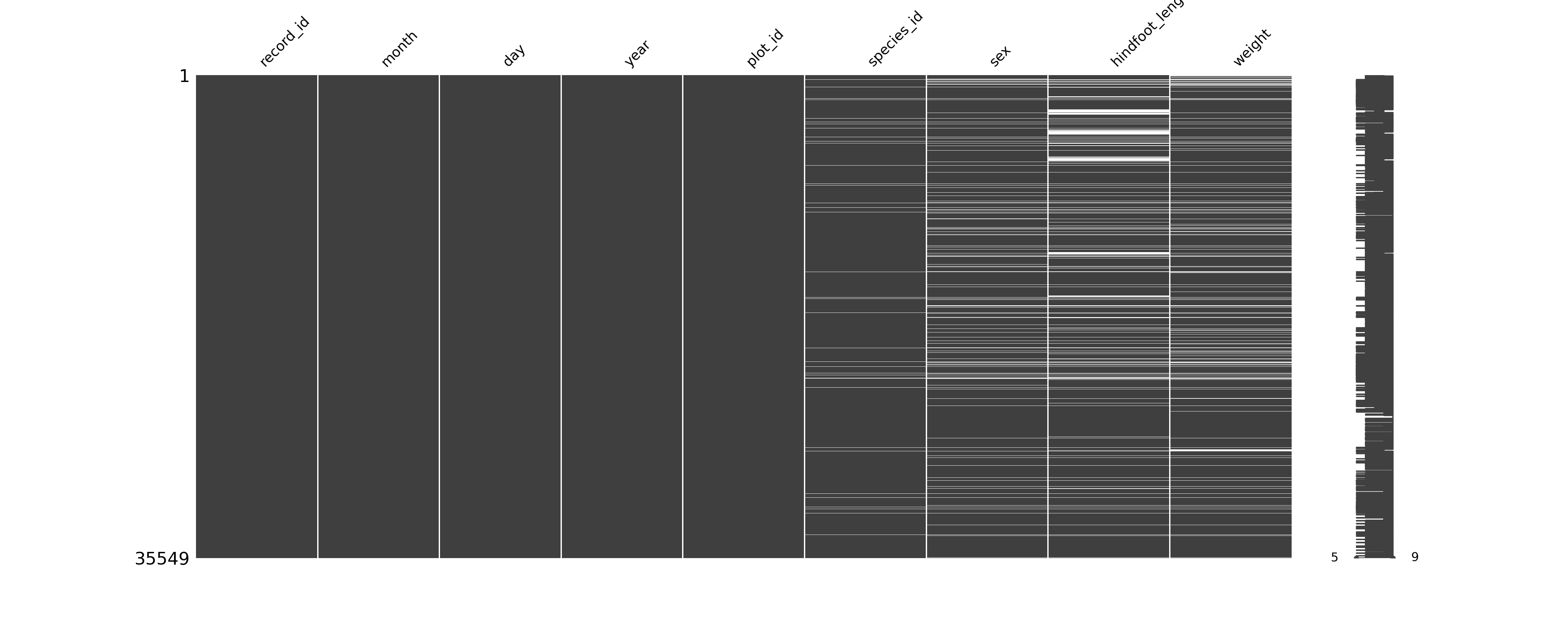
The easiest way of counting the number of missing values in Python is by combining .isna() and .sum():
# count missing values
surveys.isna().sum()
record_id 0
month 0
day 0
year 0
plot_id 0
species_id 763
sex 2511
hindfoot_length 4111
weight 3266
dtype: int64Often it’s nice to visualise where your missing values are, to see if there are any patterns that are obvious. There are several packages in Python that can do this, of which missingno is one.
import missingno as msno# visual matrix
msno.matrix(surveys)
10.7 Exercises
10.7.1 Filtering data: infections
10.7.2 Creating categories: risk_group
10.8 Summary
TipKey points
- We use the
arrange()function to order data, and can reverse the order usingdesc(). - Unique rows can be retained with
distinct(). - We use
filter()to choose rows based on conditions. - Conditions can be set using several operators:
>,>=,<,<=,==,!=,%in%. - Conditions can be combined using
&(AND) and|(OR). - The function
is.na()can be used to identify missing values. It can be negated as!is.na()to find non-missing values. - We can visualise missing data using the
vis_dat()function from thevisdatpackage.
- We can use the
.sort_values()method to order data, specifying theascending =argument asTrueorFalseto control the order. - The
.drop_duplicates()method allows us to retain unique rows. - We use subsetting (e.g.
surveys[surveys["hindfoot_length"] > 31]) together with conditions to filter data. – Conditions can be set using several operators:>,>=,<,<=,==,!=,.isin([...]). - Conditions can be combined using
&(AND) and|(OR). - The function
.isna()can be used to identify missing values. It can be negated using~to find non-missing values (e.g.surveys[~surveys["weight"].isna()]. - We can visualise missing data using the
msno.matrixfunction from themissingnopackage.