10  EQA (Exercise)

Learning Objectives

This section is an extended self-paced practice applying the concepts covered in previous sections.

By the end of this practice, you should be able to:

• Prepare all the files necessary to run the consensus pipeline.
• Run the viralrecon pipeline to generate FASTA consensus from raw FASTQ files.
• Assess and collect several quality metrics for the consensus sequences.
• Clean output files, in preparation for other downstream analysis.
• Assign sequences to lineages.
• Contextualise your sequences in other background data and cluster them based on phylogenetic analysis.
• Integrate the metadata and analysis results to generate timeseries visualisations of your data.

External Quality Assessment (EQA) is a procedure that allows laboratories to assess the quality of the data they produce, including its analysis. For genomic analysis of SARS-CoV-2, a standard panel of samples has been developed by the GenQA consortium, which is part of UK NEQAS, a non-profit that designs EQA protocols for a range of applications. GenQA’s panel of samples includes lab-cultured SARS-CoV-2 samples of known origin, enabling laboratories to assess whether their sequencing and bioinformatic pipelines correctly identify expected mutations and lineage assignments for each of the samples in the panel.

More about EQA

EQA programs such as this one help to provide assurance of the diagnostic testing results obtained by a lab. One of the key things to consider is that, for reliable assessment, samples should be processed in the same way as patient samples. Since these samples are for quality assessment, it may be tempting to assign the samples to more experienced staff, include extra checks, increase sequencing, etc. However, doing that would give a false impression of the performance of your own lab.

Evaluating the results of EQA sample processing is critical for labs to understand where their procedures can be improved. This may include staff training, purchase of new equipment, or updating the reagents and kits used for sample processing.

EQA panels are often updated, to reflect any new and emerging pathogens, allowing the labs to assess the suitability of the protocols used to detect them. It also helps raise awareness of any atypical variants of pathogens that may exist in the environment.

In this case study, we are going to analyse samples from the GenQA panel, to helps us assess the quality of our bioinformatic analysis and extract key pieces of information to be reported. Two panels are available, which include the following variants:

UKNEQAS22**

• 1x Alpha
• 1x Beta
• 1x Delta
• 2x Gamma
• 1x Omicron

UKNEQAS23**

• 2x Omicron BA.1
• 1x Omicron BA.2
• 2x Delta
• 1x Gamma

From the sequencing data analysis, we will address the following:

• What was the quality of the consensus sequence obtained?
• What lineage/clade was each of our samples assigned to? Did we identify the correct (expected) lineage?
• Which of the expected mutations were we able to detect? Where there any “false positives” or “false negatives”?

We should also produce several essential output files, which would usually be necessary to upload our data to public repositories:

• Consensus sequences (FASTA)
• Metadata and consensus sequence quality metrics (TSV)
• Variants (TSV)

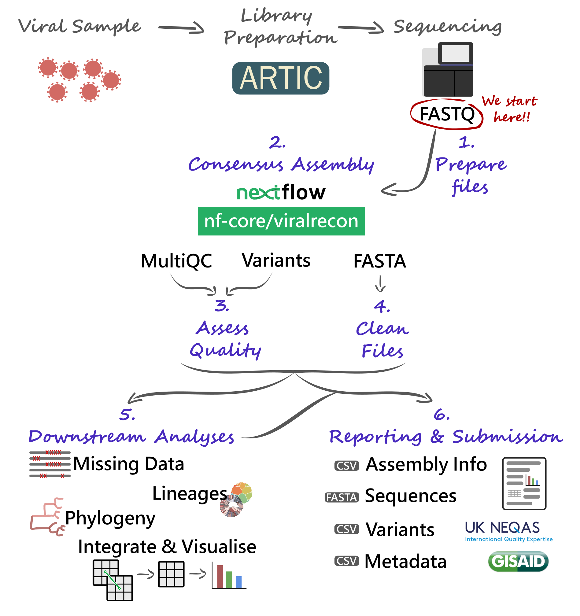
10.1 Pipeline Overview

We will start our analysis with FASTQ files produced by our sequencing platforms (Illumina and Nanopore are considered here). These FASTQ files will be used with the nf-core/viralrecon Nextflow pipeline, allowing us to automate the generation of consensus sequences and produce several quality control metrics essential for our downstream analysis and reporting.

Critical files output by the pipeline will need to be further processed, including combining and cleaning our consensus FASTA files. Using these clean files, we can then proceed to downstream analysis, which includes assigning each sample to the most up-to-date Pango lineage, Nextclade clade and WHO designation. Finally, we can do more advanced analysis, including the idenfication of sample clusters based on phylogenetic analysis, or produce timeseries visualisations of variants of concern. With all this information together, we will have the necessary pieces to submit our results to public repositories and write reports to inform public health decisions.

10.2 Preparing Files

Before we start our work, it’s always a good idea to setup our directory structure, so we keep our files organised as the analysis progresses. There is no standard way to do this, but here are some suggested directories:

• data → contains the sequencing data for the particular run or project you are working on. Data may sometimes be stored in a separate server, in which case you may not need to create this directory. Generally, you should leave the original data unmodified, in case something goes wrong during your analysis, you can always re-run it from the start.
• results → to save results of the analysis.
• scripts → to save scripts used to run the analysis. You should always try to save all the commands you run in a script, this way you will have a record of what was done to produce the results, and it makes your life easier if you want to run the analysis again on a new set of data.
• report → to save the final files and documents that we report to our colleagues or upload to public repositories.
• resources → files that you download from the internet could be saved here. For example, the reference genome sequence, background data used for phylogenetics, etc. Sometimes you may share these resources across multiple projects, in which case you could have this folder somewhere else that you can access across multiple projects.

On our computers, we have a directory in ~/Documents/eqa_workshop, where we will do all our analysis. We already include the following:

• data → with the results of the EQA sample sequencing.
• resources → where we include the SARS-CoV-2 reference genome, and some background datasets that will be used with some of the tools we will cover.
• scripts → where we include some scripts that we will use towards the end of the workshop. You should also create several scripts during the workshop, which you will save here.
• sample_info.csv → a table with some metadata for our samples.

Exercise

Your first task is to create two new directories in the project folder called report and results. You can do this either using the file explorer or from the command line (using the mkdir command).

10.2.1 Data

Regardless of which platform you used to sequence your samples, the analysis starts with FASTQ files (if you need a reminder of what a FASTQ file is, look at the Introduction to NGS section). However, the organisation of these files is slightly different depending on the platform, and is detailed below.

Nanopore

Typically, Nanopore data is converted to FASTQ format using the program Guppy. This software outputs the files to a directory called fastq_pass. Within this directory, it creates further sub-directories for each sample barcode, which are named barcodeXX (XX is the barcode number). Finally, within each barcode directory there is one (or sometimes more) FASTQ files corresponding to that sample.

You can look at the files you have available from the command line using:

ls data/fastq_pass

Illumina

The Illumina files come as compressed FASTQ files (.fq.gz format) and there’s two files per sample, corresponding to read 1 and read 2. This is indicated by the file name suffix:

• *_1.fq.gz for read 1
• *_2.fq.gz for read 2

You can look at the files you have available from the command line using:

ls data/

10.2.2 Metadata

A critical step in any analysis is to make sure that our samples have all the relevant metadata associated with them. This is important to make sense of our results and produce informative reports at the end. There are many types of information that can be collected from each sample (revise the Genomic Surveillance > Metadata section of the materials to learn more about this). For effective genomic surveillance, we need at the very minimum three pieces of information:

• When: date when the sample was collected (not when it was sequenced!).
• Where: the location where the sample was collected (not where it was sequenced!).
• How: how the sample was sequenced (sequencing platform and protocol used).

Of course, this is the minimum metadata we need for a useful analysis. However, the more information you collect about each sample, the more questions you can ask from your data – so always remember to record as much information as possible for each sample.

Exercise

Note: If you are using our pre-sequenced data, you can skip this exercise.

We already provide some basic metadata for these samples in the file sample_info.csv:

• sample → the sample ID.
• collection_date → the date of collection for the sample in the format YYYY-MM-DD.
• country → the country of origin for this sample.
• expected_lineage and expected_voc → because we are using the EQA panel, we know what lineage and variant-of-concern (VOC) each sample belongs to. We will use this later to assess the quality of our analysis.

There is however some information missing from this table, which you may have available at this point. Open this file in Excel and create the following columns:

• ct → Ct value from qPCR viral load quantification.
• sequencing_instrument → the model for the sequencing instrument used (e.g. NovaSeq 6000, MinION, etc.).
• sequencing_protocol_name → the type of protocol used to prepare the samples (e.g. ARTIC).
• amplicon_primer_scheme → for amplicon protocols, what version of the primers was used (e.g. V3, V4.1)
• Specific columns for Oxford Nanopore data, which are essential for the bioinformatic analysis:
  • ont_nanopore → the version of the pores used (e.g. 9.4.1 or 10.4.1).
  • ont_guppy_version → the version of the Guppy software used for basecalling.
  • ont_guppy_mode → the basecalling mode used with Guppy (usually “fast”, “high”, “sup” or “hac”).

This will ensure that in the future people have sufficient information to re-run the analysis on your data.

Dates in Spreadsheet Programs

Note that programs such as Excel often convert date columns to their own format, and this can cause problems when analysing data later on. For example, GISAID wants dates in the format YYYY-MM-DD, but by default Excel displays dates as DD/MM/YYYY.
You can change how Excel displays dates by highlighting the date column, right-clicking and selecting Format cells, then select “Date” and pick the format that matches YYYY-MM-DD. However, every time you open the CSV file, Excel annoyingly converts it back to its default format!

To make sure no date information is lost due to Excel’s behaviour, it’s a good idea to store information about year, month and day in separate columns (stored just as regular numbers).

10.3 Consensus Assembly

At this point we are ready to start our analysis with the first step: generating a consensus genome for our samples. We will use a standardised pipeline called viralrecon, which automates most of this process for us, helping us be more efficient and reproducible in our analysis.

Note

See Section 4.1, if you need to revise how the nf-core/viralrecon pipeline works.

10.3.1 Samplesheet

The first step in this process is to prepare a CSV file with information about our sequencing files, which will be used as the input to the viralrecon pipeline.
The pipeline’s documentation gives details about the format of this samplesheet, depending on whether you are working with Illumina or Nanopore data.

Exercise

Note: If you are using our pre-sequenced data, you can skip this exercise.

Using Excel, produce the input samplesheet for nf-core/viralrecon, making sure that you save it as a CSV file (File → Save As… and choose “CSV” as the file format).

Note: make sure that the sample names you use in this samplesheet match those in the metadata sample_info.csv file (pay attention to things like spaces, uppercase/lowercase, etc. – make sure the names used match exactly).

If you are working with Illumina data, you should check the tip below.

Illumina samplesheet: saving time with the command line!

You can save some time (and a lot of typing!) in making the Illumina samplesheet using the command line to get a list of file paths. For example, if your files are saved in a folder called data, you could do:

# list read 1 files and save output in a temporary file
ls data/*_1.fq.gz > read1_filenames.txt

# list read 2 files and save output in a temporary file
ls data/*_2.fq.gz > read2_filenames.txt

# initiate a file with column names
echo "fastq_1,fastq_2" > samplesheet.csv

# paste the two temporary files together, using comma as a delimiter
paste -d "," read1_filenames.txt read2_filenames.txt >> samplesheet.csv

# remove the two temporary files
rm read1_filenames.txt read2_filenames.txt

Now, you can open this file in Excel and continue editing it to add a new column of sample names.

10.3.2 Running Viralrecon

The next step in our analysis is to run the nf-core/viralrecon pipeline. The way the command is structured depends on which kind of data we are working with. There are many options that can be used to customise the pipeline, but typical commands are shown below for each platform.

Nanopore

nextflow run nf-core/viralrecon \
  -r 2.6.0 -profile singularity \
  --max_memory '15.GB' --max_cpus 4 \
  --platform nanopore \
  --input SAMPLESHEET_CSV \
  --fastq_dir data/fastq_pass/ \
  --outdir results/viralrecon \
  --protocol amplicon \
  --genome 'MN908947.3' \
  --primer_set artic \
  --primer_set_version PRIMER_VERSION \
  --artic_minion_caller medaka \
  --artic_minion_medaka_model MEDAKA_MODEL \
  --skip_assembly --skip_asciigenome \
  --skip_pangolin --skip_nextclade

You need to check which model the medaka software should use to process the data. You need three pieces of information to determine this:

• The version of the nanopores used (usually 9.4.1 or 10.4.1).
• The sequencing device model (MinION, GridION or PromethION).
• The mode used in the Guppy software for basecalling (“fast”, “high”, “sup” or “hac”).
• The version of the Guppy software.

Once you have these pieces of information, you can see how the model is specified based on the model files available on the medaka GitHub repository. For example, if you used a flowcell with chemistry 9.4.1, sequenced on a MinION using the “fast” algorithm on Guppy version 5.0.7, the model used should be r941_min_fast_g507.
Note that in some cases there is no model for recent versions of Guppy, in which case you use the version for the latest version available. In our example, if our version of Guppy was 6.1.5 we would use the same model above, since that’s the most recent one available.

Illumina

nextflow run nf-core/viralrecon \
  -r 2.6.0 -profile singularity \
  --max_memory '15.GB' --max_cpus 4 \
  --platform illumina \
  --input SAMPLESHEET_CSV \
  --outdir results/viralrecon \
  --protocol amplicon \
  --genome 'MN908947.3' \
  --primer_set artic \
  --primer_set_version PRIMER_VERSION \
  --skip_assembly --skip_asciigenome \
  --skip_pangolin --skip_nextclade

Exercise

Your next task is to run the pipeline on your data. However, rather than run the command directly from the command line, let’s save it in a shell script – for reproducibility and as a form of documenting our analysis.

• First, open the README.txt file found in your folder, which has some details about your samples, including the amplicon primer scheme used.
• Using a text editor, create a new shell script and save it in scripts/01-run_viralrecon.sh. You can either use the command-line text editor nano or use Gedit, which comes installed with Ubuntu.
• Copy the command shown above (either Illumina or Nanopore, depending on your data) to your new script.
• Adjust the code, to use the correct input samplesheet file, primer scheme and, in the case of ONT, the medaka model. For information about primer scheme options see the “Amplicon Primer Schemes” appendix.
• Activate the software environment to use Nextflow: mamba activate nextflow.
• Save the script and run it from the command line using bash scripts/01-run_viralrecon.sh.

If you need a reminder of how to work with shell scripts, revise the Shell Scripts section of the accompanying Unix materials.

Maximum Memory and CPUs

In our Nextflow command above we have set --max_memory '15.GB' --max_cpus 8 to limit the resources used in the analysis. This is suitable for the computers we are using in this workshop. However, make sure to set these options to the maximum resources available on the computer where you process your data.

10.4 Consensus Quality

Once your workflow is complete, it’s time to assess the quality of the assembly.

Note

See Section 5.2, if you need to revise how to assess the quality of consensus sequences.

10.4.1 Coverage

At this stage we want to identify issues such as:

• Any samples which have critically low coverage. There is no defined threshold, but samples with less than 85% coverage should be considered carefully.
• Any problematic regions that systematically did not get amplified (amplicon dropout).

Exercise

To assess the quality of our assemblies, we can use the MultiQC report generated by the pipeline, which compiles several pieces of information about our samples. If you need a reminder of where to find this file, consult the “Consensus assembly” section of the materials, or the Viralrecon output documentation.

Open the quality report and try to answer the following questions:

• Were there any samples with more than 15% missing bases (’N’s)?
• Were there any samples with a median depth of coverage <20x?
• Were there any problematic amplicons with low depth of coverage across multiple samples?

Make a note of any samples that you think are problematic. You can discuss with your colleagues and compare your results/conclusions to see if you reach similar conclusions.

10.4.2 Variants

The viralrecon pipeline outputs a table with information about SNP/Indel variants as a CSV file named variants_long_table.csv. It is important to inspect the results of this file, to identify any mutations with severe effects on annotated proteins, or identify samples with an abnormal high number of “mixed” bases.

Exercise

Open the variants_long_table.csv file and answer the following questions. If you need a reminder of where to find this file, consult the “Consensus assembly” section of the materials, or the Viralrecon output documentation.

• How many variants have allele frequency < 75%?
• Does any of the samples have a particularly high number of these low-frequency variants, compared to other samples? (This could indicate cross-contamination of samples)
• Investigate if there are any samples with frameshift mutations. These mutations should be rare because they are highly disruptive to the functioning of the virus. So, their occurrence may be due to errors rather than a true mutation and it’s good to make a note of this.

If you need a reminder of the meaning of the columns in this file, consult the Consensus > Mutation/Variant Analysis section of the materials.

Make a note of any samples that you think may be problematic, either because they have a high number of low-frequency variants or because they have frameshift mutations.

(Optional)
If you identify samples with frameshift mutations, open the BAM file of the sample using the software IGV. Go to the position where the mutation is located, and try to see if there is evidence that this mutation is an error (for example, if it’s near an homopolymer).

Exercise

The samples we are using in this analysis come from a standard EQA panel. As such, we already know what lineages we expect to find in these samples.

• Open IGV and load one (or more) of the alignment BAM files into it. If you need a reminder of where to find this file, consult the “Consensus assembly” section of the materials, or the Viralrecon output documentation.
• Open your metadata table (sample_info.csv) and check which lineages your loaded samples belong to.
• Do a web search to find what mutations characterise those lineages.
• On IGV, go to the location of some of the expected mutations, and see if you can see it in the respective samples.

10.4.3 Clean FASTA

The viralrecon pipeline outputs each of our consensus sequences as individual FASTA files for each sample (look at the FASTA Files section if you need a reminder of what these files are). However, by default, the sample names in this file have extra information added to them, which makes some downstream analysis less friendly (because the names will be too long and complicated).

To clean up these files, we will do two things:

• Combine all the individual FASTA files together.
• Remove the extra text from the sequence names.

Exercise

We will use the programs cat (concatenate) and sed (text replacement) to clean our FASTA files. Consider the commands given below:

Nanopore

cat <INPUT> | sed 's|/ARTIC/medaka MN908947.3||' > report/consensus.fa

Illumina

cat <INPUT> | sed 's| MN908947.3||' > report/consensus.fa

The sed command shown is used to remove the extra pieces of text added by the pipeline to each sample name. This is a slightly more advanced program to use, so we already give you the code. If you want to learn more about it, check the “Text Replacement” section of the accompanying Unix materials.

Copy the command above to a new shell script called scripts/02-clean_fasta.sh. Fix the code by replacing <INPUT> with the path to all the FASTA files generated by the pipeline (remember you can use the * wildcard).
If you need a reminder of where to find the FASTA consensus files from viralrecon, consult the “Consensus assembly” section of the materials, or the Viralrecon output documentation.

Once you fixed the script, run it with bash and check that the output file is generated.

Bonus:
Check that you have all expected sequences in your FASTA file using grep to find the lines of the file with > (which is used to indicate sample names).

10.4.4 Missing Intervals

When we generate our consensus assembly, there are regions for which we did not have enough information (e.g. due to amplicon dropout) or where there were mixed bases. These regions are missing data, and are denoted as ‘N’ in our sequences. Although we already determined the percentage of each sequence that is missing from the MultiQC report, we don’t have the intervals of missing data, which can be a useful quality metric to have. In particular, we may want to know what is the largest continuous stretch of missing data in each sample.

Exercise

We will use the software tool seqkit to find intervals where the ‘N’ character occurs. This tool has several functions available, one of which is called locate.

Here is the command that would be used to locate intervals containing one or more ‘N’ characters:

seqkit locate -i -P -G -M -r -p "N+" report/consensus.fa

The meaning of the options is detailed in seqkit’s documentation.

• Create a new shell script called scripts/03-missing_intervals.sh.
• Copy the command shown above to the script and modify it to redirect the output (using >) to a file called results/missing_intervals.tsv.
• Activate the software environment: mamba activate seqkit.
• Run the script you created using bash.

Exercise

Open the file you created in the previous step (results/missing_intervals.tsv) in a spreadsheet program. Create a new column with the length of each interval (end - start + 1).

Note if any missing intervals are larger than 1Kb, and whether they overlap with the Spike gene. (Note: you can use the Sars-CoV-2 genome browser to help you see the location of the annotated genes.)

10.5 Downstream Analyses

Now that we have cleaned our FASTA file, we can use it for several downstream analysis. We will focus on these:

• Lineage assignment: identify if our samples come from known lineages from the Pangolin consortium.
• Phylogeny: produce an annotated phylogenetic tree of our samples.
• Clustering: assess how many clusters of sequences we have, based on a phylogenetic analysis.
• Integration & Visualisation: cross-reference different results tables and produce visualisations of how variants changed over time.

10.5.1 Lineage Assignment

Note

See Section 6.1, if you need to revise how lineage assignment works.

Although the Viralrecon pipeline can run Pangolin and Nextclade, it does not use the latest version of these programs (because lineages evolve so fast, the nomenclature constantly changes). Although it is possible to configure viralrecon to use more recent versions of these tools, it requires more advanced use of configuration files with the pipeline.

Alternatively, we can run our consensus sequences through the latest versions of Nextclade and Pangolin. There are two ways to do this: using their respective web applications, or their command-line versions. For this task, we recommend that you use the command line tools (this will ensure our downstream analysis works well), but we also provide the option to use the web apps for your reference.

Command line

To run the command-line version of these tools, there are two steps:

• Update the datasets of each software (to ensure they are using the latest lineage/clade nomenclature available).
• Run the actual analysis on your samples.

We will use the exercises below to see what the commands to achieve this are.

Exercise

We will start doing the Nextclade analysis.

• Create a new script file called scripts/04-nextclade.sh and copy this code into it:

  # update nextclade data
  nextclade dataset get --name sars-cov-2 --output-dir resources/nextclade_background_data
  
  # run nextclade
  nextclade run --input-dataset resources/nextclade_background_data/ --output-all results/nextclade/ <INPUT>

• Fix the code, replacing <INPUT> with the path to your consensus sequence file. Save the file.

• Activate the software environment: mamba activate nextclade.

• Run your script using bash.

• Once the analysis completes, open the file results/nextclade/nextclade.tsv in Excel and see what problems your samples may have (in particular those classified as “bad” quality).

Exercise

For the Pangolin analysis:

• Create a new script file called scripts/04-pangolin.sh and copy this code into it:

  # update pangolin data
  <DATA_UPDATE_COMMAND>
  
  # run pangolin
  pangolin --outdir results/pangolin/ --outfile pango_report.csv <INPUT>

• Fix the code:

  • Replace <INPUT> with the path to your consensus sequence file.
  • Replace <DATA_UPDATE_COMMAND> with the pangolin command used to update its data. Check the documentation of the tool with pangolin --help to see if you can find what this option is called. Alternatively, look at the documentation online.

• Save the file.

• Activate the software environment: mamba activate pangolin.

• Run your script using bash.

• Once the analysis completes, open the file results/pangolin/pango_report.csv in Excel and see if there were any samples for which the analysis failed. If there were any failed samples, check if they match the report from Nextclade.

Web Apps

These exercises are optional - during the workshop please use the command line version of the tools.

Exercise

Running Nextclade

Go to clades.nextstrain.org and run Nextclade on the clean FASTA file you created earlier (report/consensus.fa).
If you need a reminder about this tool, see the “Lineages and variants” section of the materials.

Once the analysis completes, pay particular attention to the quality control column, to see what problems your samples may have (in particular those classified as “bad” quality).

Then:

• Create a new folder in your project directory: results/nextclade.
• Use the “download” button (top-right) and download the file nextclade.tsv (tab-delimited file), which contains the results of the analysis. Important: please download the TSV file (not the CSV file, as it uses ; to separate columns, and will not work later with the “Data Integration” section).
• Save this file in the results/nextclade folder you created.

Exercise

Running Pangolin

Go to pangolin.cog-uk.io and run Pangolin on the clean FASTA file you created earlier (report/consensus.fa).
If you need a reminder about this tool, see the “Lineages and variants” section of the materials.

Once the analysis completes, pay particular attention to any samples that failed. If there were any failed samples, check if they match the report from Nextclade.

Then:

• Create a new folder in your project directory: results/pangolin.
• Use the “download” button (the “arrow down” symbol on the results table) and download the file results.csv. Rename this file to report.csv (important: make sure to rename the file like this, otherwise it will not work later with the “Data Integration” section).
• Save this file in the results/pangolin folder you created.

10.5.2 Phylogeny

Note

See Section 7.1, if you need to revise how to build phylogenetic trees.

Although tools such as Nextclade and civet can place our samples in a phylogeny, sometimes it may be convenient to build our own phylogenies. This requires three steps:

• Producing a multiple sequence alignment from all consensus sequences.
• Tree inference.
• Tree visualisation.

Exercise

• Start by creating two directories to store the output of our analysis: results/mafft and results/iqtree.
• Activate the software environment: mamba activate phylo (this environment includes both mafft and iqtree).
• To make our analysis more interesting, we will combine our sequences with sequences from previous workshops. Use the cat program to concatenate your sequences (report/consensus.fa) with the sequences from our collaborators (resources/eqa_collaborators/eqa_consensus.fa). Using >, save the output in a new file results/mafft/unaligned_consensus.fa.
• Perform a multiple sequence alignment of the combined consensus sequences using the program mafft (see Section 7.2 for how to use this program). Save the output in a file called results/mafft/aligned_consensus.fa.
• Infer a phylogenetic tree using the iqtree2 program (see Section 7.3).
• Once you have both of these commands working, make sure to save them in a new shell script (as a record of your analysis). Save the script as scripts/05-phylogeny.sh.
• Visualise the tree using FigTree (see Section 7.4).

What substitution model was chosen as the best for your data by IQ-Tree?

Do your samples group with samples from previous workshops in the way that is expected, or are there any outliers?

Are there any obvious differences between sequencing technologies?

10.5.3 Clustering (Optional Section)

The software civet (Cluster Investigation and Virus Epidemiology Tool) can be used to produce a report on the phylogenetic relationship between viral samples, using a background dataset to contextualise them (e.g. a global or regional sample of sequences) as well as metadata information to enable the identification of emerging clusters of samples.

Civet works in several stages, in summary:

• Each input sequence is assigned to a “catchment” group. These are groups of samples that occur at a given genetic distance (number of SNP differences) from each other.
• Within each catchment group, a phylogeny is built (using the iqtree2 software with the HKY substitution model).
• The phylogeny is annotated with user-input metadata (e.g. location, collection date, etc.). The results are displayed in an interactive HTML report.

One of the critical pieces of information needed by civet is the background data, to which the input samples will be compared with. These background data could be anything the user wants, but typically it’s a good idea to use samples from the local geographic area from where the samples were collected. For example, a national centre may choose to have their background data composed of all the samples that have been sequenced in the country so far. Or perhaps all the samples in its country and other neighbouring countries.

One way to obtain background data is to download it from GISAID. An example of how to do this is detailed in the civet documentation. We have already downloaded the data from GISAID, so we can go straight to running our civet analysis.

Exercise

• Create a new script in scripts/06-civet.sh, with the following command, adjusted to fit your files:

  civet -i <PATH_TO_YOUR_SAMPLE_METADATA> \
    -f <PATH_TO_YOUR_CONSENSUS_FASTA> \
    -icol <COLUMN_NAME_FOR_YOUR_SAMPLE_IDS> \
    -idate <COLUMN_NAME_FOR_YOUR_COLLECTION_DATE> \
    -d <PATH_TO_CIVET_BACKGROUND_DATA> \
    -o results/civet

• Activate the software environment: mamba activate civet.

• Once your script is ready, run it with bash.

• After the analysis completes, open the HTML output file in results/civet and examine into how many catchments your samples were grouped into.

10.6 Integration & Visualisation

At this point in our analysis, we have several tables with different pieces of information:

• sample_info.csv → the original table with metadata for our samples.
• results/viralrecon/multiqc/medaka/summary_variants_metrics_mqc.csv → quality metrics from the MultiQC report generated by the viralrecon pipeline.
• results/nextclade/nextclade.tsv → the results from Nextclade.
• results/pangolin/pango_report.csv → the results from Pangolin.
• (optional) results/civet/master_metadata.csv → the results from the civet analysis, namely the catchment (or cluster) that each of our samples was grouped into.

Each of these tables stores different pieces of information, and it would be great if we could integrate them together, to facilitate their interpration and generate some visualisations.

We will demonstrate how this analysis can be done using the R software, which is a popular programming language used for data analysis and visualisation. Check the Quick R Intro appendix for the basics of how to work with R and RStudio.

Exercise

Data Integration

From RStudio, open the script in scripts/07-data_integration.R. Run the code in the script, going line by line (remember in RStudio you can run code from the script panel using Ctrl + Enter). As you run the code check the tables that are created (in your “Environment” panel on the top-right) and see if they were correctly imported.

Once you reach the end of the script, you should have two tab-delimited files named report/consensus_metrics.tsv and report/variants.tsv. Open both files in Excel to check their content and confirm they contain information from across the multiple tables.

Exercise

Data Visualisation

After integrating the data, it’s time to produce some visualisations. From RStudio, open the script in scripts/08-visualisation.R. Run the code in the script, going line by line.

As you run the code, several plots will be created. You can export these plots from within RStudio using the “Export” button on the plotting panel – these will be useful when you write your report later.

Exercise

Annotating Phylogenetic Tree

Using FigTree, import two annotation files (File > Import Annotations…):

• report/consensus_metrics.tsv, which was created in the Data Integration exercise.
• resources/eqa_collaborators/metadata.tsv, which has lineage assignment for EQA samples sequenced by other labs.

After importing both files, annotate your phylogenetic tree to display the lineages assigned to each sample as the tip labels. See Section 7.4, if you need a reminder of how to annotate trees using FigTree.

10.7 EQA Panels

The analysis we have done so far is applicable to any new sequences that you want to process. However, we have also been using a pre-defined panel of samples to be used as part of an External Quality Assessment (EQA) process. This allows us to assess whether our bioinformatic analysis identified all the expected mutations in these samples, as well as assigned them to the correct lineages.

To do this, requires to compare the mutations we detected in our EQA samples to the expected mutations provided to us. From this, we will be able to calculate True Positives (TP), False Positives (FP) and False Negatives (FN), and calculate two performance metrics:

• Precision = TP / (TP + FP) → what fraction of the mutations we detected are true?
• Sensitivity = TP / (TP + FN) → what fraction of all true mutations did we detect?

There can be cases where one of these metrics is high and the other one lower. For example, if you have a high-coverage genome (say >95%) but lots of sequencing errors, you may have a high sensitivity (you manage to detect all true mutations), but low precision (you also detect lots of false positives, due to sequencing errors). Conversely, if you have a low-coverage genome (say <50%) but very high-quality sequencing, you may have low sensitivity (you missed lots of true mutations, because of missing data), but high precision (those mutations that you did manage to identify were all true, you didn’t have many false positives).

If you are submiting your samples to GenQA’s platform, they will also provide with a general accuracy score called F-score. This is calculated as the harmonic mean of precision and sensitivity:

\(F_{score} = \frac{2 \times Precision \times Sensitivity}{Precision + Sensitivity}\)

A high F-score is indicative of both high precision and sensitivity, whereas a lower score indicates that at least one of those metrics are low.

Exercise

From RStudio, open the script in scripts/09-eqa_validation.R. Run the code in the script, going line by line.

This script will save a new tab-delimited file in report/eqa_performance_metrics.tsv. Open this file in Excel and check what the precision and sensitivity of your analysis was. Are you happy with the results?

Exercise

(Optional)

While you run the R script, you will have an object called all_mutations in your environment (check the top-right panel). From RStudio, click on the name of this object to open it in the table viewer.

Look at mutations that were not detected in your samples, but were present in the expected mutations (i.e. false negatives). Open the BAM file for one of those samples in IGV and navigate to the position where that mutation should occur. Investigate what the reason may have been for missing that mutation.

If you need a reminder of where to find the BAM file, consult the Consensus > Output Files section of the materials, or the Viralrecon output documentation.

10.8 Reporting

Finally, we have come to the end of our analysis. So, all that is left is to report our results in the most informative way to our colleagues and decision-makers. You may already have established reporting templates in your institution, and if that’s the case, you should use those. Alternatively, we will look at a suggested template, based on the reports done by the UK Health Security Agency (UKHSA).

Exercise

Open our shared report template document and download it as a Word document (File → Download → Microsoft Word (.docx)). Save the file in report/YYYY-MM-DD_analysis_report.docx (replace YYYY-MM-DD by today’s date).

Open the file and complete it with the information you collected throughout your analysis. You should be able to get all this information from the files in your report/ directory.