7 Building phylogenetic trees

Learning Objectives

Understand the basics of how phylogeny trees are constructed using maximum likelihood methods.
Describe what branch lengths represent in typical SARS-CoV-2 phylogenetic tree.
Recognise the limitations and challenges in building phylogenies for SARS-CoV-2.
Use MAFFT to produce a multiple sequence alignment.
Use IQ-Tree for phylogenetic tree inference.
Use TimeTree to obtain time-scaled phylogenetic trees using sample collection date metadata.

7.1 SARS-CoV-2 Phylogeny

Global Phylogeny

Building phylogenetic trees for SARS-CoV-2 is challenging due to the large number of sequences available, with millions of genomes submited to GISAID to this day. This means that using maximum-likelihood inference tools to build a global SARS-CoV-2 phylogeny is both time-consuming and computationally demanding.

However, several researchers have dedicated their time to identifying tools and models suitable for the phylogenetic analysis of this organism. For example, the global phylogenies repository from Rob Lanfear provide with several tips on building phylogenetic trees for this organism. Their trees are regularly updated and available to download from the GISAID website (which requires an account).

Global phylogenies are also available from the groups of Russell Corbett-Detig and Yatish Turakhia, who have developed efficient methods and tools for dealing with large phylogenies. These tools include UShER and matUtils, introducing a new and efficient file format for storing phylogenetic trees, mutations and other annotations (such as lineages) called mutation-annotated trees (MAT format). Their phylogenies are updated daily and are publicly available for download. (Note: Course materials covering these tools are still under development.)

Two popular tools used for phylogenetic inference via maximum-likelihood are FastTree and IQ-Tree. Generally, when building a tree from a collection of samples you can include the Wuhan-Hu-1 reference sequence as an outgroup to root the tree. Optionally, you can also add a collection of sequences from around the world (and across time) to contextualise your samples in the global diversity.

As an input, these programs need a multiple sequence alignment FASTA file, which is where we start our analysis.

Data for this section

We will work from the course materials folder called 04-phylogeny, which contains the following files:

data/uk_consensus.fa and data/india_consensus.fa are consensus sequences from the UK and India, respectively. These are the sequences previously assembled using the nf-core/viralrecon pipeline.
sample_annotation.tsv is a tab-separated values (TSV) file with information about each sample such as the date of collection and lineage/clade they were assiged to from our analysis. We will use this table to annotate our phylogenetic trees. This table can also be opened in a spreadsheet program such as Excel.
resources/reference/sarscov2.fa is the reference genome.

7.2 Alignment

The first step in building a phylogenetic tree is to produce a multiple sequence alignment from all our consensus sequences. This is the basis for building a phylogenetic tree from the positions that are variable across samples.

A widely used multiple sequence alignment software is called MAFFT. For SARS-CoV-2, a reference-based alignment approach is often used, which is suitable for closely-related genomes. MAFF provides this functionality, which is detailed in its documentation.

We demonstrate the analysis using the UK samples in our course materials. First, start by creating a directory for the output:

mkdir -p results/mafft

Then, we run the command to generate a reference-based alignment:

mafft --6merpair --maxambiguous 0.2 --addfragments data/uk_consensus.fa resources/reference/sarscov2.fa > results/mafft/uk_alignment.fa

The meaning of the options used is:

--6merpair is a fast method for estimating the distances between sequences, based on the number of short 6bp sequences shared between each pair of sequences. This is less accurate than other options available (like --localpair and --globalpair), but runs much faster in whole genome data like we have.
--maxambiguous 0.2 automatically removes samples with more than 20% ambiguous ‘N’ bases (or any other value of our choice). This is a convenient way to remove samples with poor genome coverage from our analysis.
--addfragments data/consensus_sequences.fa is the FASTA file with the sequences we want to align.
finally, at the end of the command we give the reference genome as the input sequence to align our sequences against.

MAFFT provides several other methods for alignment, with tradeoffs between speed and accuracy. You can look at the full documentation using mafft --man (mafft --help will give a shorter description of the main options). For example, from its documentation we can see that the most precise alignment can be obtained with the options --localpair --maxiterate 1000. However, this is quite slow and may not be feasible for whole genome data of SARS-CoV-2.

7.2.1 Visualising alignments

We can visualise our alignment using the software AliView, which is both lightweight and fast, making it ideal for large alignments. Visualising the alignment can be useful for example to identify regions with missing data (more about this below).

Snapshop of an alignment visualised with AliView. In this case we are looking at the end of the alignment of our sequences, which shows a typical high number of missing (‘N’) bases.

Other Alignment Strategies

There are other commonly used alignment tools used for SARS-CoV-2 genomes:

The minimap2 software has been designed for aligning long sequences to a reference genome. It can therefore be used to align each consensus sequence to the Wuhan-Hu-1 genome. This is the tool internally used by Pangolin.
Nextclade uses an internal alignment algorithm where each consensus sequence is aligned with the reference genome. The alignment produced from this tool can also be used for phylogenetic inference.

It is worth mentioning that when doing reference-based alignment, insertions relative to the reference genome are not considered.

7.3 Tree Inference: IQ-Tree

IQ-TREE supports many substitution models, including models with rate heterogeneity across sites.

Let’s start by creating an output directory for our results:

mkdir -p results/iqtree

And then run the program with default options (we set --prefix to ensure output files go to the directory we just created and are named “uk”):

iqtree2 -s results/mafft/uk_alignment.fa --prefix results/iqtree/uk

Without specifying any options, iqtree2 uses ModelFinder to find the substituion model that maximizes the likelihood of the data, while at the same time taking into account the complexity of each model (using information criteria metrics commonly used to assess statistical models).

From the information printed on the console after running the command, we can see that the chosen model for our alignment was “GTR+F+I”, a generalised time reversible (GTR) substitution model. This model requires an estimate of each base frequency in the population of samples, which in this case is estimated by simply counting the frequencies of each base from the alignment (this is indicated by “+F” in the model name). Finally, the model includes rate heterogeneity across sites, allowing for a proportion of invariant sites (indicated by “+I” in the model name). This makes sense, since we know that there are a lot of positions in the genome where there is no variation in our samples.

We can look at the output folder (specified with --prefix) where we see several files with the following extension:

.iqtree - a text file containing a report of the IQ-Tree run, including a representation of the tree in text format.
.treefile - the estimated tree in NEWICK format. We can use this file with other programs, such as FigTree, to visualise our tree.
.log - the log file containing the messages that were also printed on the screen.
.bionj - the initial tree estimated by neighbour joining (NEWICK format).
.mldist - the maximum likelihood distances between every pair of sequences.
ckp.gz - this is a “checkpoint” file, which IQ-Tree uses to resume a run in case it was interrupted (e.g. if you are estimating very large trees and your job fails half-way through).
.model.gz - this is also a “checkpoint” file for the model testing step.

The main files of interest are the report file (.iqtree) and the NEWICK tree file (.treefile).

Inference of very large trees

Although running IQ-Tree with default options is fine for most applications, there will be some bottlenecks once the number of samples becomes too large. In particular, the ModelFinder step may be very slow and so it’s best to set a model of our choice based on other people’s work. For example, work by Rob Lanfear suggests that models such as “GTR+G” and “GTR+I” are suitable for SARS-CoV-2. We can specify the model used by iqtree2 by adding the option -m GTR+G, for example.

For very large trees (over 10k or 100k samples), using an alternative method to place samples in an existing phylogeny may be more adequate. UShER is a popular tool that can be used to this end. It uses a parsimony-based method, which tends to perform well for SARS-CoV-2 phylogenies.

7.4 Visualising Trees

There are many programs that can be used to visualise phylogenetic trees. In this course we will use FigTree, which has a simple graphical user interface.

To open the tree, go to File > Open… and browse to the folder with the IQ-Tree output files. Select the file with .treefile extension and click Open. You will be presented with a visual representation of the tree.

We can also import a “tab-separated values” (TSV) file with annotations to add to the tree. For example, we can use our results from Pangolin and Nextclade, as well as other metadata to improve our visualisation (we have prepared a TSV with this information combined, which you could do using Excel or another spreadsheet software).

Go to File > Import annotations… and open the annotation file.
On the menu on the left, click Tip Labels and under “Display” choose one of the fields of our metadata table. For example, you can display the lineage assigned by Pangolin (“pango_lineage” column of our annotation table).

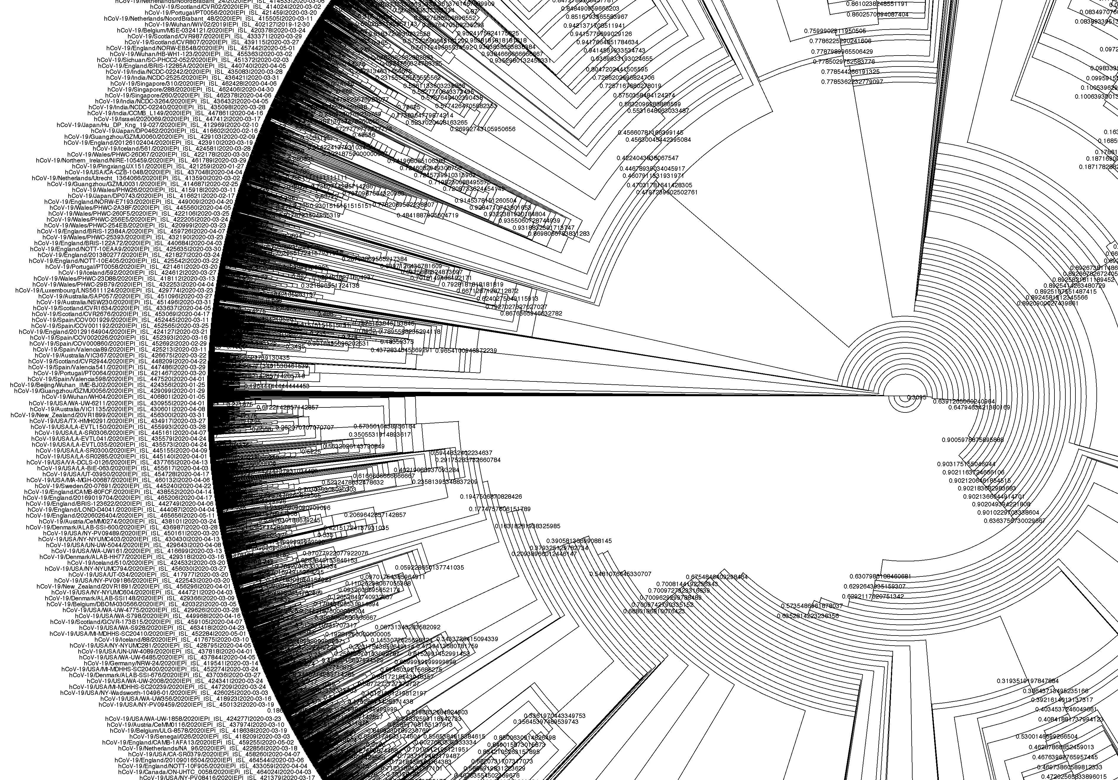
There are many ways to further configure the tree, including highlighting clades in the tree, and change the labels. See the figure below for an example.

Annotated phylogenetic tree obtained with FigTree. We used the lineage of each sample as our tip labels and aligned the labels on the right (check the tickbox at the top of the left menu called “Align tip labels”). We identified two clades in the tree that corresponded to the Alpha and Delta variants, and used the “Highlight” tool to give them different colours. To do this, change the “Selection Mode” at the top to “Clade”, then select the branch at the base of the clade you want to highlight, and press the “Highlight” button on the top to pick a colour.

7.5 Time-scaled Phylogenies

The trees that we build from sequence data are scaled using the mutation rate estimated from the sequence alignments. This is useful if we want to know, for example, on average how many mutations separate different branches of the tree.

Another way to scale trees is to use time. For viral genome sequences, we usually have information about their date of collection, and this can be used to scale the phylogeny using the date information. The idea is to rescale the trees such that the x-axis of the tree represents a date rather than number of mutations.

Two programs that can be used to time-scale trees using date information are called TreeTime and Chronumental. Chronumental was developed for dealing with very large phylogenies (millions of samples), but lacks some of the functionalities provided by TreeTime (such as estimating uncertainty in date estimates, reconstructing past sequences, re-rooting trees, among others). So, if you are working with less than ~50,000 sequences, we recommend using TreeTime, otherwise Chronumental is a suitable alternative.

Because we are dealing with a small number of samples, we will show an example of using TreeTime to scale our tree based on our dates:

treetime --tree results/iqtree/uk.treefile --dates sample_annotation.tsv --aln results/mafft/uk_alignment.fa --outdir results/treetime/uk

After running, this tool produces several output files in the specified folder. The main files of interest are:

timetree.nexus is the new date-scaled tree. NEXUS is another tree file format, which can store more information about the tree compared to the simpler NEWICK format. This format is also supported by FigTree.
timetree.pdf is a PDF file with the inferred tree, including a time scale on the x-axis. This can be useful for quick visualisation of the tree.

We can visualise this tree in FigTree, by opening the file timetree.nexus. The scale of this new tree now corresponds to years (instead of nucleotide substitution rates). We make make several adjustments to this tree, to make it look how we prefer. For example:

Label the nodes of the tree with the inferred dates: from the left menu click Node Labels and under “Display” select “date”.
Import the metadata table (sample_annotation.tsv file) and display the results of Nextclade or Pangolin clades/lineages.
Adjust the scale of the tree to be more intuitive. For example, instead of having the unit of the scale in years, we can change it to months. On the left menu, click Time Scale and change “Scale factor” to 12 (twelve months in a year). Then click Scale Bar and change the “Scale range” to 1. The scale now represents 1 month of time, which may be easier to interpret in this case.

Note that there is uncertainty in the estimates of the internal node dates from TimeTree and these should be interpreted with some caution. The inference of the internal nodes will be better the more samples we have, and across a wider range of times. In our specific case we had samples all from a similar period of time, which makes our dating of internal nodes a little poorer than might be desired.

More precise tree dating may be achieved by using public sequences across a range of times or by collecting more samples over time. Time-scaled trees of this sort can therefore be useful to infer if there is a recent spread of a new clade in the population.

7.6 Missing Data & Problematic Sites

So far, we have been using all of our assembled samples in the phylogenetic analysis. However, we know that some of these have poorer quality (for example the “IN01” sample from India had low genome coverage). Although, generally speaking, sequences with missing data are unlikely to substantially affect the phylogenetic results, their placement in the phylogeny will be more uncertain (since several variable sites may be missing data). Therefore, for phylogenetic analysis, it is best if we remove samples with low sequencing coverage, and instead focus on high-quality samples (e.g. with >80% coverage).

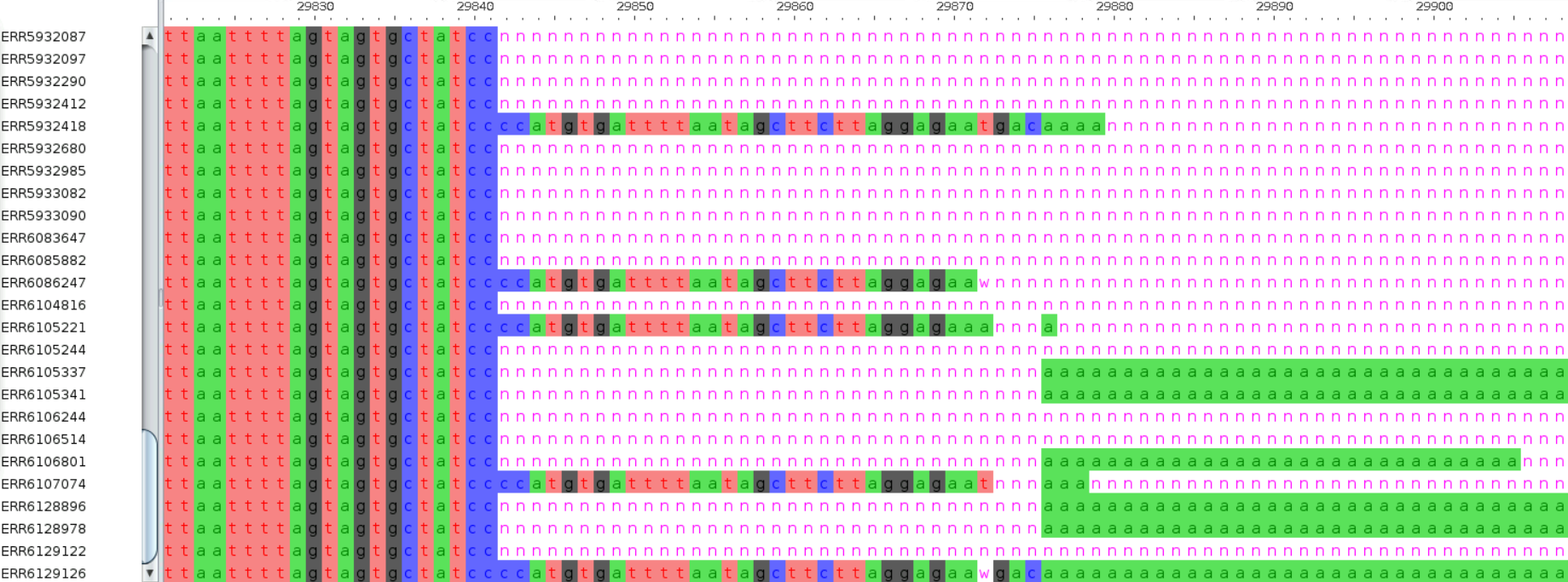
A more serious issue affecting phylogenies is the presence of recurrent errors in certain positions of the genome. One of the regions with a higher prevalence of errors is the start and end of the consensus sequence, which also typically contains many missing data (see example in Figure 2). Therefore, it is common to mask the first and last few bases of the alignment, to avoid including spurious variable sites in the analysis.

Sequence masking

The term masking is often used to refer to the process of converting sequence bases to the ambiguous character ‘N’. You may come across this term in the documentation of certain tools, for example: “Positions with less than 20x depth of sequencing are masked.”

Masks are not limited to depth of sequencing. For example, reference genomes from ENSEMBL are available with masked repeat or low-complexity sequences (e.g. around centromeres, transposon-rich regions, etc.).

The term soft masking is also used to refer to cases where, instead of using the ambiguous character ‘N’, sequences are masked with a lowercase. For example:

>seq_with_soft_masking
ACAGACTGACGCTGTcatgtatgtcgacGATAGGCTGATGGCGAGTGACTCGAG
>seq_with_hard_masking
ACAGACTGACGCTGTNNNNNNNNNNNNNGATAGGCTGATGGCGAGTGACTCGAG

Additionally, work by Turakhia, de Maio, Thornlow, et al. (2020) has identified several sites that show an unexpected mutation pattern. This includes, for example, mutations that unexpectedly occur multiple times in different parts of the tree (homoplasies) and often coincide with primer binding sites (from amplicon-based protocols) and can even be lab-specific (e.g. due to their protocols and data processing pipelines). The work from this team has led to the creation of a list of problematic sites, which are recommended to be masked before running the phylogenetic analysis.

Example of errors in phylogenetic inference due to recurrent sequencing errors. Source: Figure 1 in Turakhia, de Maio, Thornlow et al. (2020)

So, let’s try to improve our alignment by masking the problematic sites, which are provided as a VCF file. This file also includes the first and last positions of the genome as targets for masking (positions 1–55 and 29804–29903, relative to the Wuhan-Hu-1 reference genome MN908947.3). The authors also provide a python script for masking a multiple sequence alignment. We have already downloaded these files to our course materials folder, so we can go ahead and use the script to mask our file:

python scripts/mask_alignment_using_vcf.py --mask -v resources/problematic_sites.vcf -i results/mafft/uk_alignment.fa -o results/mafft/uk_alignment_masked.fa

If we open the output file with AliView, we can confirm that the positions specified in the VCF file have now been masked with the missing ‘N’ character.

We could then use this masked alignment for our tree-inference, just as we did before.

Using Python Scripts

Bioinformaticians often write custom scripts for particular tasks. In this example, the authors of the “problematic sites” wrote a Python script that takes as input the FASTA file we want to mask as well as a VCF with the list of sites to be masked.

Python scripts are usually run with the python program and often accept options in a similar way to other command-line tools, using the syntax --option (this is not always the case, but most professionally written scripts follow this convention). To see how to use the script we can use the option --help. For our case, we could run:

python scripts/mask_alignment_using_vcf.py --help

7.7 Exercises

Building phylogenies

So far we have focused our analysis on the samples from the UK. In this exercise you will be able to practice these steps on the samples from India. The steps are similar to what we have done so far, and you can consult the materials in the sections above to go through each exercise.

In the following exercises, you can run the commands directly from the command line. But if you feel comfortable with nano, as a bonus, you can try to save the commands in a shell script.

Using mafft, produce a multiple-sequence alignment from the India consensus sequences in the file data/india_consensus.fa. Save the output in a file named results/mafft/india_alignment.fa.
Using iqtree2, infer a phylogenetic tree from this alignment. Save the output with prefix results/iqtree/india.
- What substitution model did IQ-Tree infer as the most likely for the data?
Using FigTree, visualise the inferred tree:
- Open the .tree output file.
- Import the annotation table sample_annotation.tsv.
- Make the tip labels display the Nextclade clade instead of the sample names.
- Highlight any clusters of the tree containing WHO variants of concern.
Using timetree, re-scale the phylogeny using dates (the file sample_annotation.tsv can be used as input to timetree along with the previously-created phylogeny and alignments). Output the result to results/treetime/india
- Open the .nexus output file in FigTree.
- Make the node labels display the date inferred by timetree.
Two samples in the time-scaled tree appear at the root of the tree: IN05 and IN33. But we would have expected the reference sample (MN908947.3) to be the root of the tree, as it was collected in Dec 2019.
- Investigate what lineages these samples were assigned to.
- Go to https://cov-lineages.org/lineage_list.html and check when those lineages were detected.
- Is the collection date metadata for these samples compatible with the lineage information from the Pangolin website? Can you hypothesise what may have happened with these samples?

Answer

Question 1

We run our alignment using the following command:

mafft --6merpair --maxambiguous 0.2 --addfragments data/india_consensus.fa resources/reference/sarscov2.fa > results/mafft/india_alignment.fa

We could optionally visualise our alignment using AliView to check that the alignment was successful.

Question 2

We can fit a maximum-likelihood tree using the following command:

iqtree2 -s results/mafft/india_alignment.fa --prefix results/iqtree/india

This command prints a lot of output on the screen. We can see all this information (and more!) on the output file results/iqtree/india.iqtree, which contains a log of all the analysis done by the program. We could, for example, use the less program to look inside this file. When we do this, we can see the following:

ModelFinder
-----------

Best-fit model according to BIC: GTR+F+I

Which indicates that the substitution model used by IQ-Tree was “GTR+F+I”. This is the same model that was determined for the UK samples, and an explanation of this model is given in the materials above.

Question 3

Using FigTree:

Go to File > Open… and browse to the folder with the IQ-Tree output files.
Select the file with india.treefile and click Open.
Go to File > Import annotations… and open the annotation file sample_annotation.tsv.
On the menu on the left, click Tip Labels and under “Display” choose the field “nextclade_clade”.

On this tree, there is a small group of samples classified as “20I (Alpha; V1)”. These samples correspond to the Alpha variant of concern. To highlight these:

Change the “Selection Mode” at the top to “Clade”.
Select the branch corresponding to the base of the group of samples classified as Alpha. This should highlight all those branches.
Click the “Highlight” button at the top and choose a colour.

Question 4

The command to time-scale the tree is:

treetime --tree results/iqtree/india.treefile --dates sample_annotation.tsv --aln results/mafft/india_alignment.fa --outdir results/treetime/india

Once complete, we can open the india.nexus tree with FigTree. We can annotate the internal nodes of the tree with the dates inferred by treetime by clicking on the Node Labels menu on the left and selecting “Display” to be “date”.

Question 5

To investigate this strange result, we open the sample_annotation.tsv file in our spreadsheet program. We can see the following information for these two samples:

name    date           country  year     month  pango_lineage      nextclade_clade
IN05    2021-01-21   India    2021   1      A.23.1           19B
IN33    2021-01-21   India    2021   1      A.23.1           19B

Both these samples were assigned to Pango lineage “A.23.1”. From the cov-lineages.org website we can see that these were detected as early as 2020-06-08.

However, our samples’ metadata indicate that these samples were collected in January 2021, that is 7 months after these samples were first detected globally.

This contractiction explains the strange result in our time-scaled tree. These samples will have mutations that are part of the older lineage “A”, but were annotated to be from 2021. So treetime put them down at the root of the tree.

This discrepancy could indicate an issue with the metadata collection, which perhaps is wrong. For example, it could be that these samples were collected months before January 2021, but only sequenced then. And by mistake the date of sequencing was recorded as the date of collection.

This is an example how important accurate metadata is for our analysis.

7.8 Summary

Key Points

Methods for phylogenetic inference include parsimony and maximum likelihood. Maximum likelihood methods are preferred because they include more features of the evolutionary process. However, they are computationally more demanding than parsimony-based methods.
To build a phylogenetic tree we need a multiple sequence alignment of the sequences we want to infer a tree from.
In SARS-CoV-2, alignments are usually done against the Wuhan-Hu-1 reference genome.
We can use the software mafft to produce a multiple sequence alignment. The option --addfragments is used to produce an alignment against the reference genome.
The software iqtree2 can be used for inferring trees from an alignment using maximum likelihood. This software supports a wide range of substitution models and a method to identify the model that maximizes the likelihood of the data.
Some of the substituion models that have been used to build global SARS-CoV-2 phylogenies are “GTR+G” and “GTR+I”.
We can time-scale trees using sample collection date information. The program treetime can be used to achieve this. For very large sample sizes (>50,000 samples) the much faster program Chronumental can be used instead.
Before building a phylogeny, we should be careful to mask problematic sites that can lead to misleading placements of samples in the tree. The SARS-CoV-2 Problematic Sites repository provides with an updated list of sites that should be masked.