8 Switzerland (Nanopore)

Learning Objectives

This section demonstrates a start-to-finish analysis of a dataset sequenced on a Nanopore platform, using the concepts and tools covered in previous sections. You can download the data from these links (two versions available):

Switzerland Case Study - Full Data – this includes data for 65 samples, which gives a more realistic sample size, but can take several hours to run on a small computer.
Switzerland Case Study - Small Version – this includes data for a subset of 10 samples, which is more suitable for training purposes (but the results will look slightly different from the ones shown here).

By the end of this section, you should be able to:

Prepare all the files necessary to run the consensus pipeline.
Run the viralrecon pipeline to generate FASTA consensus from raw FASTQ files.
Assess and collect several quality metrics for the consensus sequences.
Clean output files, in preparation for other downstream analysis.
Assign sequences to lineages using Nextclade and/or Pangolin.
Contextualise your sequences in other background data and cluster them based on phylogenetic analysis.
Integrate the metadata and results to generate useful visualisations of your data.
Report your analysis.

We will analyse data from 48 samples collected in Switzerland between Nov 2021 and Jan 2022. The samples were sequenced on a GridION platform using pore version 9.4.1.

The final product of our work (and main objective) is to produce a report of the analysis, which you can see here: Switzerland Case Study Report.

In summary, the report addresses the following:

What was the quality of the consensus sequences?
What lineage/clade was each of our samples assigned to?
How many clusters of samples did we identify?
How did the detected lineages change over the time of sampling?

We also produce several essential output files, which would usually be necessary to upload our data to public repositories:

Metadata (CSV)
Consensus sequences (FASTA)
Consensus sequence quality metrics (CSV)
Variants (CSV)

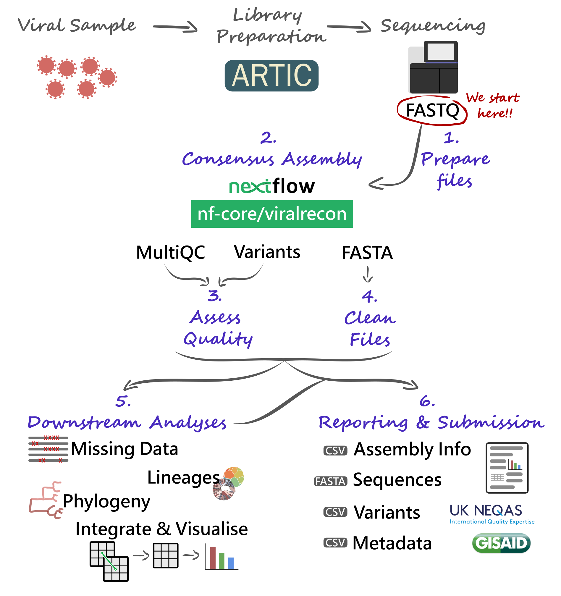
8.1 Pipeline Overview

Our analysis starts with FASTQ files, which will be used with the nf-core/viralrecon Nextflow pipeline. This will give us several quality control metrics essential for our downstream analysis and reporting.

Critical files output by the pipeline will need to be further processed, including combining our consensus FASTA files and obtaining a list of filtered SNP/indel variants. Using these clean files, we can then proceed to downstream analysis, which includes assigning each sample to the most up-to-date Pango lineage, Nextclade clade and WHO designation. Finally, we can do more advanced analysis, including the idenfication of sample clusters based on phylogenetic analysis, or produce timeseries visualisations of mutations or variants of concern. With all this information together, we will have the necessary pieces to submit our results to public repositories and write reports to inform public health decisions.

8.2 Preparing Files

Before we start our work, it’s always a good idea to setup our directory structure, so we keep our files organised as the analysis progresses. From the data we are starting with, we already have the following directories:

data → contains the sequencing data in a sub-directory called fast_pass.
resources → files that were downloaded from public repositories.
scripts → bash and R scripts used to run the analysis.

We create two additional directories:

report → files and documents that we report to our colleagues or upload to public repositories.
results → results of the analysis.

You can create directories from the command line using the mkdir command:

mkdir results
mkdir report

8.2.1 Data

We start our analysis from FASTQ files generated using the software Guppy v6.1.5 ran in “fast” mode. This software outputs the files to a directory called fastq_pass, with further sub-directories for each sample barcode. This is how it looks like in this case:

ls data/fastq_pass

barcode01  barcode08  barcode15  barcode22  barcode29  barcode36  barcode43  barcode50  barcode57
barcode02  barcode09  barcode16  barcode23  barcode30  barcode37  barcode44  barcode51  barcode58
barcode03  barcode10  barcode17  barcode24  barcode31  barcode38  barcode45  barcode52  barcode59
barcode04  barcode11  barcode18  barcode25  barcode32  barcode39  barcode46  barcode53  barcode60
barcode05  barcode12  barcode19  barcode26  barcode33  barcode40  barcode47  barcode54  barcode61
barcode06  barcode13  barcode20  barcode27  barcode34  barcode41  barcode48  barcode55  barcode62
barcode07  barcode14  barcode21  barcode28  barcode35  barcode42  barcode49  barcode56  barcode63

8.2.2 Metadata

Metadata for these samples is available in the file sample_info.csv. Here is some of the information we have available for these samples:

sample → the sample ID.
collection_date → the date of collection for the sample in the format YYYY-MM-DD.
country → the country of origin for this sample.
latitude/longitude → coordinates for sample location (optional).
sequencing_instrument → the model for the sequencing instrument used (e.g. NovaSeq 6000, MinION, etc.).
sequencing_protocol_name → the type of protocol used to prepare the samples (e.g. ARTIC).
amplicon_primer_scheme → for amplicon protocols, what version of the primers was used (e.g. V3, V4.1)
Specific columns for Oxford Nanopore data, which are essential for the bioinformatic analysis:
- ont_pore → the version of the pores.
- ont_guppy_version → the version of the Guppy software used for basecalling.
- ont_guppy_mode → the basecalling mode used with Guppy.

8.3 Consensus Assembly

Note

See Section 4.1, if you need to revise how the nf-core/viralrecon pipeline works.

The first step in the bioinformatic analysis is to run the nf-core/viralrecon pipeline.

8.3.1 Samplesheet

But first we need to prepare our input files. For Nanopore data, we need a samplesheet CSV file with two columns, indicating sample name (first column) and the respective barcode number (second column).

We produced this table in Excel and saved it as a CSV file. Here are the top few rows of the file:

head samplesheet.csv

sample,barcode
CH01,1
CH02,2
CH03,3
CH04,4
CH05,5
CH06,6
CH07,7
CH08,8
CH09,9
CH10,10

8.3.2 Running Viralrecon

Now we are ready to run the nf-core/viralrecon pipeline (see Section 4.3 for details). We saved our command in a script (scripts/01-run_viralrecon.sh), which we created with the command line text editor nano. This ensures that our analysis is reproducible and traceable (we can go back to the script to see how the analysis was run).

First, we activate our software environment, to ensure Nextflow is available to us:

mamba activate nextflow

Then, we run our script with:

bash scripts/01-run_viralrecon.sh

Which will start executing the pipeline.

For reference, here is the command included in that script:

nextflow run nf-core/viralrecon \
  -r 2.6.0 -profile singularity \
  --max_memory '16.GB' --max_cpus 8 \
  --platform nanopore \
  --input samplesheet.csv \
  --fastq_dir data/fastq_pass/ \
  --outdir results/viralrecon \
  --protocol amplicon \
  --genome 'MN908947.3' \
  --primer_set artic \
  --primer_set_version 3 \
  --artic_minion_caller medaka \
  --artic_minion_medaka_model r941_min_fast_g303 \
  --skip_assembly --skip_asciigenome \
  --skip_pangolin --skip_nextclade

In this case, we used the medaka model r941_min_fast_g303, because that is the latest one available (even though our Guppy version is 6.1.5). We also restricted our --max_memory and --max_cpus due to the size of our processing computers. If a larger computer was available, we could have used higher values for these parameters.

The \ in long commands

In the command above, you will notice several \ at the end of each line. This is indicating that we want to continue writing our command in the next line. Notice that the last line does not include \, because that is the end of the command. This is very useful when commands are very long, because it makes the code more readable.

8.4 Consensus Quality

Note

See Section 5.2, if you need to revise how to assess the quality of consensus sequences.

8.4.1 General Metrics

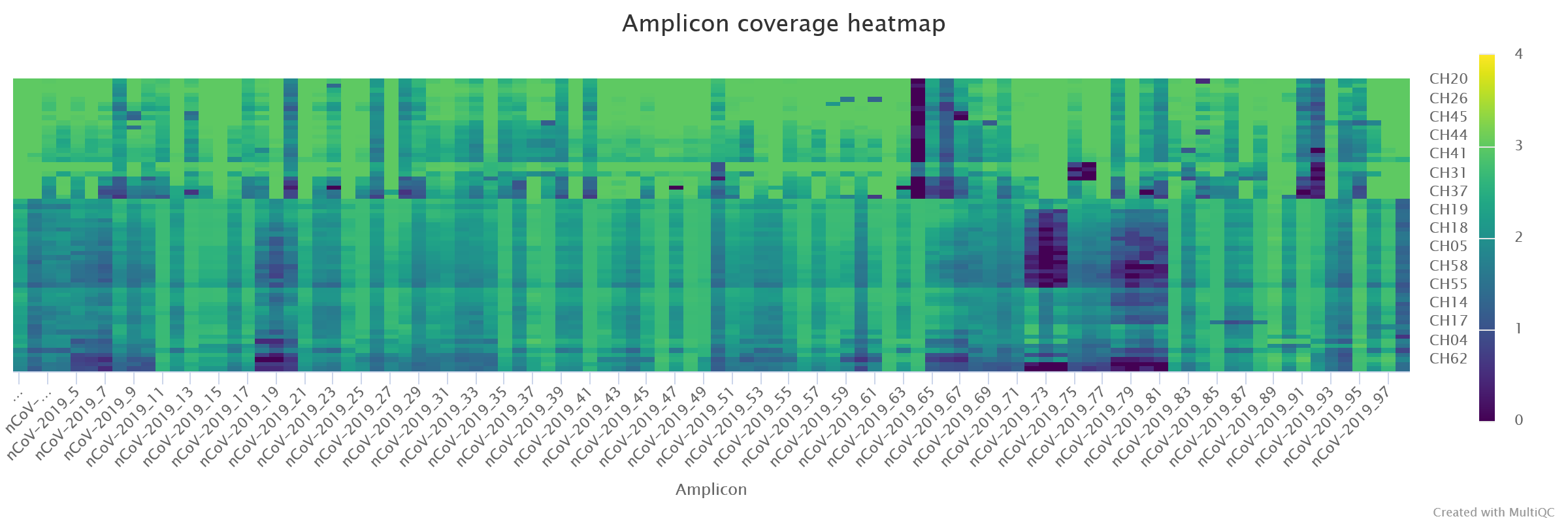
We used the MultiqQC report to assess the initial quality of our samples. The quality report can be found in results/viralrecon/multiqc/medaka/multiqc_report.html.

We paid particular attention to:

Number of reads mapped to the reference genome.
Median depth of coverage.
Percentage of the genome with missing bases (‘N’).
Number of SNP + Indel variants.

Example *MultiQC* output, highlighting the main columns with quality information that will be collected for the final report.

We noted that:

9 samples had more than 15% missing bases.
All samples had median depth of coverage greater than 20x.
There was some systematic dropout for some amplicons, in particular nCoV-2019_64 had very low amplification in several of the samples. Of note was also nCoV-2019_73, and other neighbouring amplicons.

Amplicon depth of sequencing (or coverage) across samples, from the *MultiQC* report. Darker regions indicate systematic amplicon dropout, probably due to issues during the PCR amplification.

Besides the MultiQC report, the pipeline also outputs a CSV file with collected summary metrics (equivalent to the first table on the report): results/viralrecon/multiqc/medaka/summary_variants_metrics_mqc.csv. We will use this file later to join this information with our metadata and lineage assignment using the R software (detailed in “Integration & Visualisation” section, below).

8.4.2 Variants

We also looked at the table of variants obtained from the pipeline. This is output in results/viralrecon/medaka/variants_long_table.csv. This table can be very useful to keep track of particular mutations that may be increasing over time. Later, we will tidy this table to attach to our reported results (“Integration & Visualisation” section).

But for now, we will explore this table to address a few more quality-related questions. We opened this table in Excel to answer the following:

Where there samples with a high number of intermediate allele frequencies? This could indicate mixed samples due to cross-contamination.
Where there samples with frameshift mutations? These mutations should be rare because they are highly disruptive to the functioning of the virus. So, their occurrence may be due to errors rather than a true mutation and it’s good to make a note of this.

All the variants in our samples had an alternative allele frequency (AF column) greater than 68%, which is a good indication that there were no mixed samples. We did note two samples – CH13 and CH49 – had a frameshift mutation each, in the Spike and ORF1a proteins, respectively. This may be due to a sequencing error, as it is not observed in any other samples. The inclusion of this error may not affect our downstream analysis significantly, but we make a note of these two samples, to check if their lineage assignment and phylogenetic analysis makes sense later on (or whether they appear as outliers, indicating broader sequencing quality issues).

Variants table output by *viralrecon*, with a summary of the main columns of interest. Note that this table also includes a column with lineage assignment (not shown in this snapshot). Remember that at this stage we mostly ignore this column, as *viralrecon* does not use the most up-to-date version of the lineage databases.

8.4.3 Clean FASTA

The pipeline outputs the consensus sequences in results/viralrecon/medaka/*.consensus.fasta (one file for each sample). For downstream analysis, it is convenient to combine all these sequences into a single file, and also clean the sequence names (to remove some text – “/ARTIC/medaka MN908947.3” –, which is added by the medaka variant caller).

We created a new script to clean our consensus FASTA files, which we ran with bash scripts/02-clean_fasta.sh:

#!/bin/bash 

# combine and clean FASTA files
cat results/viralrecon/medaka/*.consensus.fasta | sed 's|/ARTIC/medaka MN908947.3||' > report/consensus.fa

This command does two things:

Combine all our FASTA consensus sequences into a single file (using cat).
Clean the sequence names (using sed).

The output was saved as a new FASTA file: report/consensus.fa.

8.4.4 Missing Intervals

As a further quality check, we also generated a table of missing intervals (indicated by the N character in the FASTA sequences). We used the seqkit software to achieve this.

First, we activate our software environment:

mamba activate seqkit

Then, we ran the script bash scripts/03-missing_intervals.sh, which includes the following command:

seqkit locate -i -P -G -M -r -p "N+" report/consensus.fa > results/missing_intervals.tsv

This software outputs a tab-delimited table, which we saved as results/missing_intervals.tsv. The table looks like this (only the top few rows are shown):

seqID  patternName  pattern  strand  start  end
CH01   N+           N+       +       1      54
CH01   N+           N+       +       1193   1264
CH01   N+           N+       +       4143   4322
CH01   N+           N+       +       6248   6294
CH01   N+           N+       +       7561   7561
CH01   N+           N+       +       9243   9311
CH01   N+           N+       +       10367  10367
CH01   N+           N+       +       11361  11370
CH01   N+           N+       +       13599  13613

We opened this file missing_intervals.tsv in Excel and quickly calculated the length of each interval. We noted that two samples – CH07 and CH59 – both have a continuous interval of 5130 missing bases between positions 19580 and 24709. This includes part of the ORF1a gene and nearly all of the S (Spike) gene. This may be due to a poor amplification of one of the PCR amplicons and may affect the interpretation of the results for these two samples. We make a note of these samples as being possibly problematic in downstream analysis steps.

8.5 Downstream Analyses

Based on the clean consensus sequences, we then perform several downstream analysis.

8.5.1 Lineage Assignment

Note

See Section 6.1, if you need to revise how lineage assignment works.

Although the Viralrecon pipeline runs Pangolin and Nextclade, it does not use the latest version of these programs (because lineages evolve so fast, the nomenclature constantly changes). An up-to-date run of both of these tools can be done using each of their web applications:

However, for automation, reproducibility and traceability purposes, we used the command line versions of these tools, and included their analysis in two scripts.

Nextclade
Pangolin

For Nextclade, we first activate the software environment:

mamba activate nextclade

And then we ran the script bash scripts/04-nextclade.sh, which contains the following commands:

# get nextclade data
nextclade dataset get --name sars-cov-2 --output-dir resources/nextclade_background_data

# run nextclade
nextclade run --input-dataset resources/nextclade_background_data/ --output-all results/nextclade report/consensus.fa

The first command downloads the latest version of the Nextclade background data using nextclade dataset. We use that data as input to the second command (nextclade run) to make sure it runs with the most up-to-date lineages.

For Pangolin, we first activate the software environment:

mamba activate pangolin

And then we ran the script bash/04-pangolin.sh, which contains the following commands:

# update pangolin data
pangolin --update-data

# run pangolin
pangolin --outdir results/pangolin/ --outfile pango_report.csv report/consensus.fa

Similarly to before, we first ran pangolin --update-data to ensure we were using the latest lineages available. We can check the version of the data used with pangolin --all-versions (at the time we ran this we had pangolin-data: 1.23.1).

Both of these tools output CSV files, which can be open in Excel for further examination.
Opening the pangolin results (results/pangolin/pango_report.csv), we noticed that two samples – CH07 and CH59 – failed the QC due to high fraction of missing data. These are the same two samples that had a large gap of missing data in the previous section. Several other samples were classified as “Probable Omicron”, which from the “scorpio_notes” column we can see may be because too many of the expected mutations had missing (ambiguous) bases in those consensus sequences.
Opening the nextclade results (results/nextclade/nextclade.tsv), we noticed that 23 samples were assigned a QC status of “bad”, mostly due to high percentage of missing data (nextclade uses a stringent threshold of 3000 sites, or ~10%, missing data).

Like before, we will do further analysis (and visualisation) of these data using the software R, in the section “Integration & Visualisation”, detailed below.

8.5.2 Phylogeny

Note

See Section 7.1, if you need to revise how to build phylogenetic trees.

Although a tool such as Nextclade can place our samples in a global phylogeny context, sometimes it may be convient to build our own phylogenies. This requires three steps:

Producing a multiple sequence alignment from all consensus sequences.
Tree inference.
Tree visualisation and annotation.

Before our analysis, we first activated our software environment:

mamba activate phylo

We performed the first two steps with the following script, which we ran with bash scripts/05-phylogeny.sh:

# alignment
mkdir -p results/mafft
mafft --6merpair --maxambiguous 0.2 --addfragments report/consensus.fa resources/reference/sarscov2.fa > results/mafft/alignment.fa

# tree inference
mkdir -p results/iqtree
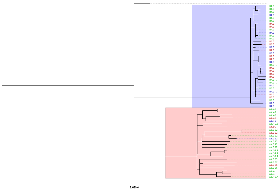
iqtree2 -s results/mafft/alignment.fa --prefix results/iqtree/consensus

The output of iqtree includes a tree file, which can be visualised using FigTree (or online using Microreact). The figure below shows an example of an annotated tree, where we highlight the main VOCs detected. This annotation was done based on the file that we generate in the next section (“Integration & Visualisation”), so those steps would have to be done first.

We can see that our samples fall broadly into two large clusters, which correlate with the VOC classification for these samples.

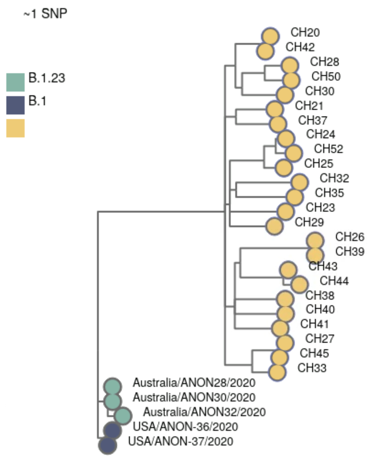
Phylogenetic tree for our samples. The top cluster (purple) highlights samples classified as Omicron (BA.1-related) and the bottom cluster (pink) samples classified as Delta (AY lineage, also known as B.1.617.2). The tips of the tree are coloured according to *Nextclade*’s QC status: green = “good”; blue = “mediocre”; red = “bad”.

8.5.3 Clustering

We identified groups of similar sequences in our data using the software civet (Cluster Investigation and Virus Epidemiology Tool). This software compares our samples with a background dataset of our choice, which givus us more context for our analysis. In this case we are using the example background data that comes with civet. However, in a real-world analysis, it would have been ideal to choose local samples as background data. For example, we could download samples from Switzerland from around the time period of our sample collection, from GISAID following the instructions on the civet documentation (you need an account on GISAID to obtain these data).

For this example, we already prepared civet background dataset saved in resources/civet_background_data.

Before our analysis, we first activate our software environment:

mamba activate civet

Then, we ran the script bash scripts/06-civet.sh, which contains the following code:

# run civet analysis
civet \
  -i sample_info.csv \
  -f report/consensus.fa \
  -icol sample \
  -idate collection_date \
  -d resources/civet_background_data/ \
  -o results/civet

The result of this analysis includes an interactive HTML report (in results/civet/civet.html). We can see that our samples were grouped into 2 catchments, using this background data. This makes sense from our previous lineage/variant analysis: the two catchments correlate with the two main variants in these data (Omicron and Delta).

Example of results from *civet* report for catchment 2, showing the phylogeny in the context of the samples in the background data (coloured according to their lineages).

Civet also outputs a CSV file (results/civet/master_metadata.csv), which includes the catchment that each sample was assigned to. We will use this CSV file later to integrate this information with other parts of our analysis, in R, detailed in the “Integration & Visualisation” section.

8.6 Integration & Visualisation

At this point in our analysis, we have several tables with different pieces of information:

sample_info.csv → the original table with metadata for our samples.
results/viralrecon/multiqc/medaka/summary_variants_metrics_mqc.csv → quality metrics from the MultiQC report generated by the viralrecon pipeline.
results/nextclade/nextclade.tsv → the results from Nextclade.
results/pangolin/pango_report.csv → the results from Pangolin.
results/civet/master_metadata.csv → the results from the civet analysis, namely the catchment (or cluster) that each of our samples was grouped into.

To consolidate our analysis, we tidied and integrated the information from across these different files, into a single table using the software R. The script used to do this is in scripts/07-data_integration.R. Because this is an R script, we opened it in RStudio to execute the code.

The output of our script is a new tab-delimited table, which we saved in report/consensus_metrics.tsv, and contains the following columns:

sample → sample ID.
collection_date → date of collection day.
collection_week → date of collection week (useful for summarising/visualising counts per-week).
country → country of origin.
latitude/longitude → latitude and longitude of collection.
n_mapped_reads → number of mapped reads.
median_depth → median depth.
pct_missing → percentage of missing data.
pct_coverage → percentage of coverage.
n_variants → number of SNP + indel variants detected.
nextclade → nextclade clade.
qc_status → QC status as determined by Nextclade (“bad”, “mediocre”, “good”).
lineage → Pangolin lineage.
who_variant → variant of concern designation.
catchment → catchment group from Civet.

This table, which aggregates information from many of the tools we used, was then used to produce different visualisations of our analysis. These visualisations were also done using the R software (scripts/08-visualisation.R), and integrated into a report, shown below.

8.7 Bonus: Full Workflow

Although we have ran each of the steps of our analysis individually (each in their own script), now that we have everything working, we could integrate all these steps into a single “master” script:

#!/bin/bash

# make mamba activate command available
eval "$(conda shell.bash hook)"
source $(mamba info --base)/etc/profile.d/mamba.sh

# make report directory
mkdir -p report

mamba activate nextflow

# run viralrecon
nextflow run nf-core/viralrecon \
  -r 2.6.0 -profile singularity \
  --max_memory '16.GB' --max_cpus 8 \
  --platform nanopore \
  --input samplesheet.csv \
  --fastq_dir data/fastq_pass/ \
  --outdir results/viralrecon \
  --protocol amplicon \
  --genome 'MN908947.3' \
  --primer_set artic \
  --primer_set_version 3 \
  --artic_minion_caller medaka \
  --artic_minion_medaka_model r941_min_fast_g303 \
  --skip_assembly --skip_asciigenome \
  --skip_pangolin --skip_nextclade

# combine and clean FASTA files
cat results/viralrecon/medaka/*.consensus.fasta | sed 's|/ARTIC/medaka MN908947.3||' > report/consensus.fa

mamba activate seqkit

# create missing bases TSV file
seqkit locate -i -P -G -M -r -p "N+" report/consensus.fa > results/missing_intervals.tsv

mamba activate nextclade

# get nextclade data
nextclade dataset get --name sars-cov-2 --output-dir resources/nextclade_background_data

# run nextclade
nextclade run --input-dataset resources/nextclade_background_data/ --output-all results/nextclade report/consensus.fa

mamba activate pangolin

# update pangolin data
pangolin --update-data

# run pangolin
pangolin --outdir results/pangolin/ --outfile pango_report.csv report/consensus.fa

mamba activate phylo

# alignment
mkdir -p results/mafft
mafft --6merpair --maxambiguous 0.2 --addfragments report/consensus.fa resources/reference/sarscov2.fa > results/mafft/alignment.fa

# tree inference
mkdir -p results/iqtree
iqtree2 -s results/mafft/alignment.fa --prefix results/iqtree/consensus

# data integration and cleaning
Rscript scripts/07-data_integration.R

Notice that we included the R script that does the data cleaning here, using the Rscript program that allows to execute an R script from the command-line.

Having this “master” script, we could run all these steps from start-to-finish with a single command, which can be very useful if you want to fully automate your analysis across multiple runs.