9 Publication-quality visualisations
- Create clear and informative molecular visualisations using ChimeraX.
- Combine structural representations such as cartoons, surfaces, and atoms.
- Adjust lighting, background, and outlines to improve figure clarity.
- Generate rotating or animated movies of molecular structures.
- Use tiled views to compare multiple structures simultaneously.
High-quality molecular visualisations are an important part of communicating structural biology results. Figures used in publications or presentations should aim to be:
- informative - highlighting the structural features relevant to the question
- clear - avoiding unnecessary clutter
- visually consistent - using colour and representation carefully
ChimeraX provides a wide range of tools for producing such figures.
The ChimeraX gallery showcases many examples of publication-quality visualisations. Each example includes a downloadable .cxc script that reproduces the image using ChimeraX commands.
Studying these scripts is often a useful way to learn new visualisation techniques.
9.1 Surface representation
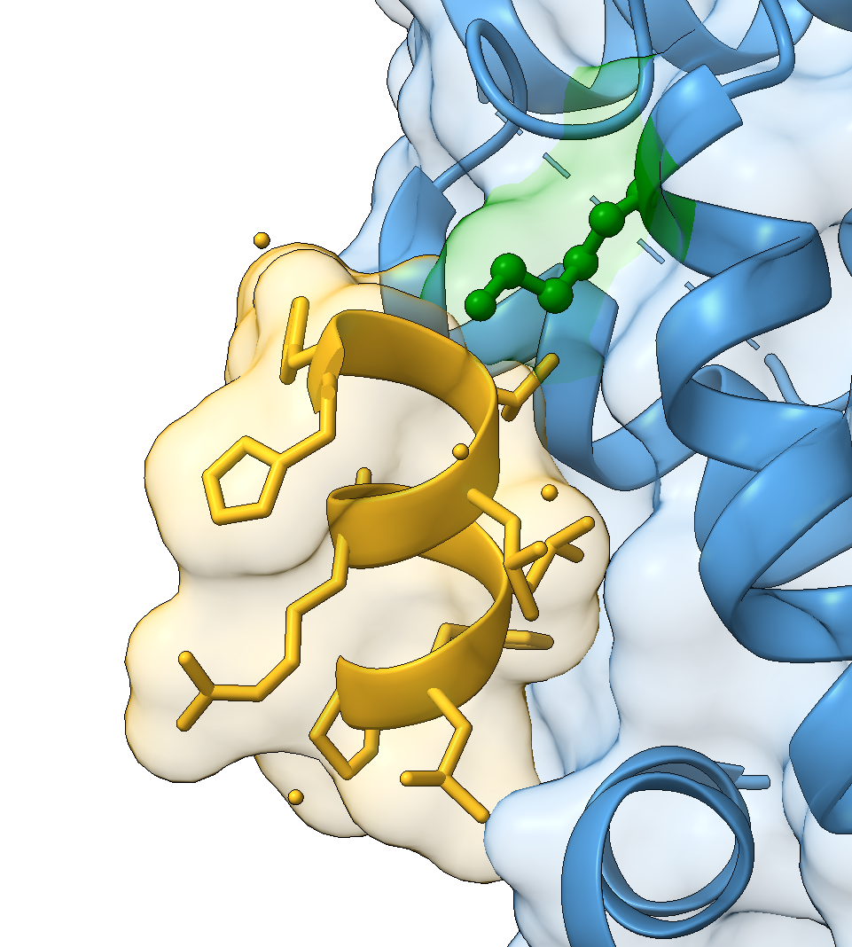
Consider the following view of the estrogen receptor in complex with a conserved peptide motif characteristic of activator proteins (PDB: 4J26).
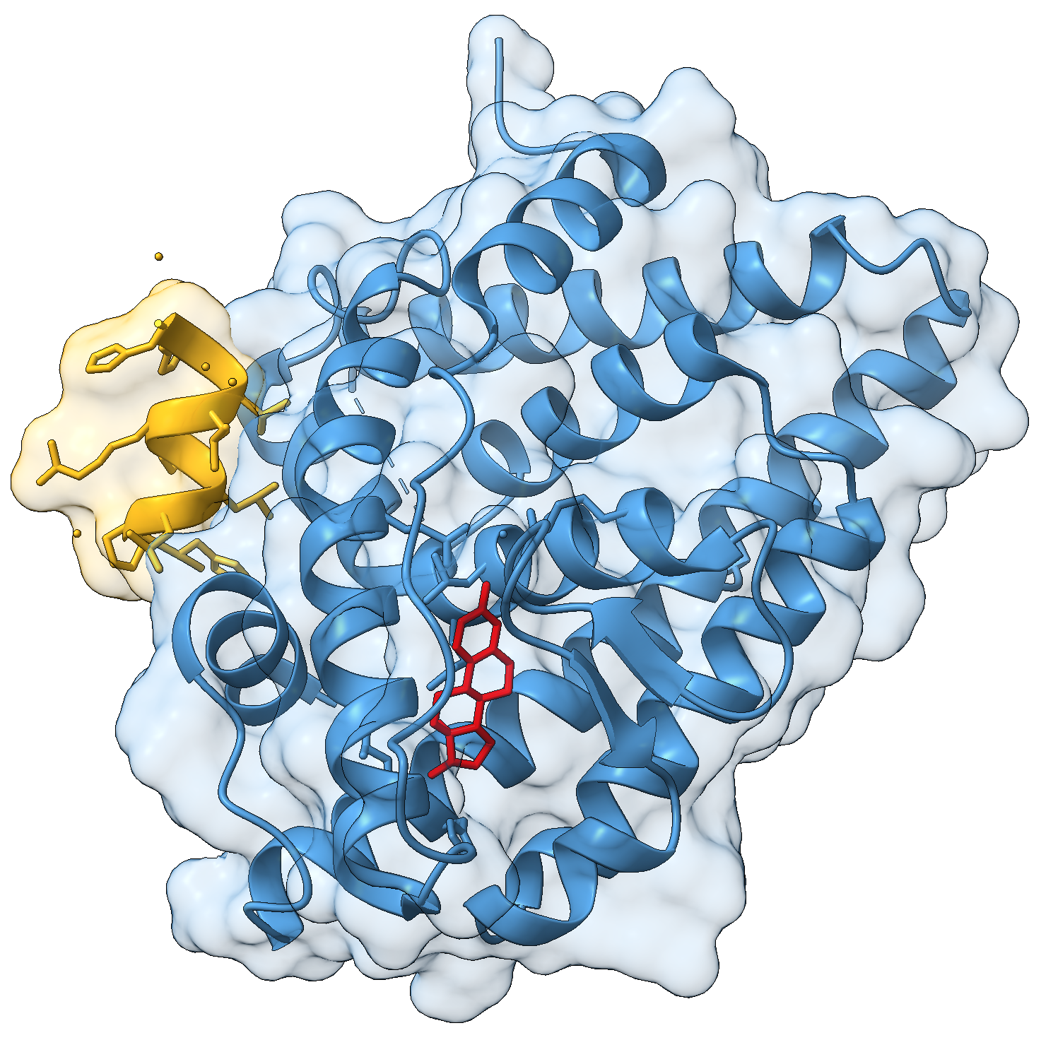
This visualisation combines several features to highlight the interaction between the receptor and the peptide.
Below are the commands used to generate the figure:
close
open 4J26
delete /A,I
set bgcolor white
label delete
light simple
graphics silhouettes true width 1
show /J atoms
color /B steelblue
color /J goldenrod
color :EST red
surface /B transparency 85
surface /J transparency 85
Let’s break these down step-by-step.
We begin by loading the structure and simplifying the model.
The crystal structure contains two receptor-peptide complexes, so we remove chains A and I to keep only one complex.
delete /A,INext we adjust the global visual settings.
set bgcolor white
label delete
light simple
graphics silhouettes true width 1
These commands:
- set a white background, which is standard for publications
- remove default residue labels
- use simple lighting to improve contrast
- add silhouettes (black outlines) around objects
Silhouettes are particularly useful because they help the structure stand out clearly against the background.
We then highlight the relevant structural components.
show /J atoms
color /B steelblue
color /J goldenrod
color :EST red
Here we:
- display the coactivator peptide atoms
- colour the receptor chain blue
- colour the peptide gold
- colour the ligand red
Using distinct colours makes it easier to identify the different molecular components.
Finally, we display transparent molecular surfaces for both chains:
surface /B transparency 85
surface /J transparency 85
The transparent surface illustrates the shape of the binding interface, while still allowing the underlying secondary structure to remain visible.
9.2 Creating a movie
Movies can help illustrate structural features that are difficult to appreciate in a static image.
ChimeraX supports several types of automatic motion:
rock- oscillating back-and-forth motionroll- continuous 360 degree rotationwobble- figure-eight style motionturn- flexible rotation around arbitrary axes
The general workflow for creating a movie is:
- start recording
- perform the desired movement
- stop recording
- encode the frames into a video file
9.2.1 Example: rocking animation
We can create a rocking animation of the estrogen receptor using:
rockTo stop the motion:
stopTo record a movie, we use the movie record command. It is helpful to record complete motion cycles, so that the movie loops smoothly.
According to the ChimeraX documentation, the default rocking motion completes one cycle in 136 frames. We therefore record one full cycle using:
movie record
rock
wait 136
stop
Finally, we encode the movie as an MP4 file:
movie encode 4j26_rock.mp4 framerate 60The framerate option determines how many frames are shown per second in the final movie.
9.3 Animated views
ChimeraX also allows you to define named views and smoothly transition between them. This approach is useful for guiding the viewer through different parts of a structure.
First we define a set of views:
- View 1: entire protein
- View 2: coactivator peptide
- View 3: ligand binding site
view protein
view name 1
view /J
view name 2
view ligand
view name 3
Each view name command stores the current camera position. We can then transition between these views while recording a movie. The syntax:
view <name> <frames>controls how long the transition takes.
For example:
view 1
movie record
view 2 60
wait 80
view 1 30
wait 30
view 3 60
wait 80
view 1 30
wait 30
movie encode 4j26_views.mp4 framerate 30
Deciding on the framerates for each view and transition can require some trial and error, but it helps to think about it in relation to the framerate used to encode the movie. In this example:
- the movie is encoded at 30 frames per second
- a transition of 60 frames corresponds to 2 seconds
- pauses are introduced using the
waitcommand
9.4 UniProt annotations
Functional annotations can also be incorporated into visualisations.
For example, we can retrieve UniProt information for the estrogen receptor. The UniProt identifier for the receptor is P03372:
open P03372 from uniprot format uniprotThis opens the sequence annotation panel, where features such as domains, mutations, and binding sites can be inspected. Selecting a feature highlights the corresponding residues in the structure.
For example, one of the mutations annotated in UniProt is described as: “K → R completely inactive in positive regulation of DNA-binding transcription factor activity”. Once selected, the residue can be highlighted in the structure:
select /B:314
show sel atoms
style sel ball
colour sel green
select clear
Highlighting biologically important residues is often helpful when preparing figures that illustrate functional mechanisms.
9.5 Tiled views
ChimeraX also supports tiled layouts, allowing multiple structures to be displayed side-by-side. This is particularly useful when comparing:
- different ligand-bound structures
- conformational states
- homologous proteins
The tile command automatically arranges open models into a grid layout. For example:
tile column 4 spacingfactor 0.8This arranges four models in a single row, with slightly reduced spacing between panels. Tiled views are frequently used in publications to compare related structures under consistent orientations.
9.6 Exercises
Create a movie of the oestrogen receptor structure rotating 360 degrees around the y-axis. Save it as a mp4 file.
Going back to our video transitioning between different views:
view 1
movie record
view 2 60
wait 80
view 1 30
wait 30
view 3 60
wait 80
view 1 30
wait 30
movie encode 4j26_views.mp4 framerate 30
Can you modify the code above, to include a rocking movement after zooming in on view 2 and view 3?

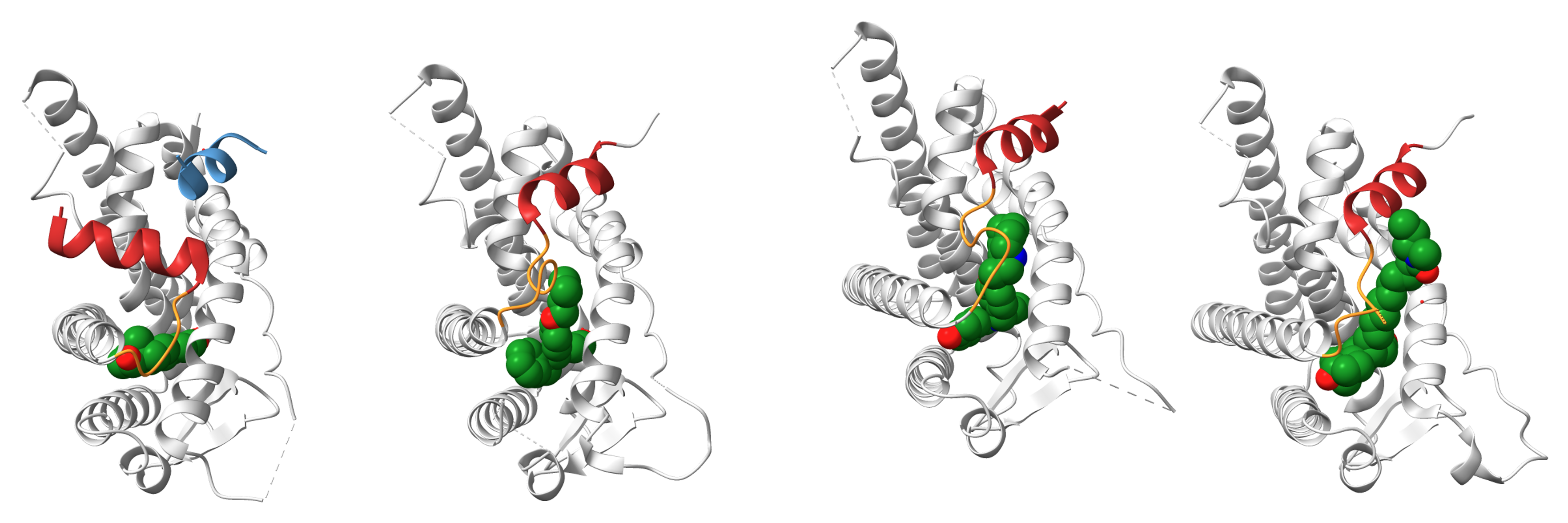
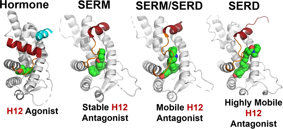
Try to recreate this view of the Oestrogen Receptor complexed with different ligands (PDBs: 1GWR, 5W9C, 4XI3, and 7R62):
- Import all the structures into a new ChimeraX session.
- These models each have multiple chains, but we will work with only chain A in each structure, plus their respective ligands, listed below. Create a selection to only show these chains and ligands, and delete the rest of the structure.
1GWR: bound to the hormone estradiol (residues named:EST); also include the coregulator peptide motif (chain/C)5W9C: bound to the tamoxifen-derived drug 4-hydroxytamoxifen (residues named:OHT)4XI3: bound to the drug bazedoxifene (residues named:29S)7R62: bound to a synthetic estradiol-like inhibitor (residues named:3YJ)
- Align the structures to each other to ensure similar orientations, and tile the views in a 1x4 grid.
- Colour the protein in silver, and the ligands by element (carbon in green, oxygen in red, and nitrogen in blue).
- Show the coregulator peptide motif in cyan.
- Use the sequence viewer to identify the positions of helix 12 in each structure, and colour it red, and the helix 11-12 loop in orange.
We start by opening the structures of interest:
close
open 1GWR
open 5W9C
open 4XI3
open 7R62
We then select chain A and the ligand for each structure, and delete the rest of the structure:
select #1/A | #1/C | #1/A:EST | #2/A | #2/A:OHT | #3/A | #3/A:29S | #4/A | #4/A:3YJ
delete ~sel
select clear
We have opted to use the OR | operator to select multiple chains and ligands at the same time, but you could also do this in multiple steps if you prefer using the select add command.
We then align the structures to each other to ensure similar orientations:
mm #2-4 to #1We tile the views using the tile command, and colour the structures using silver, similar to the original publication:
tile column 4 spacingfactor 0.8
colour protein silver
hide protein atoms
We represent the ligands as spheres, and colour them by element:
show ligand atoms
style ligand sphere
colour ligand & C green
colour ligand & O red
colour ligand & N blue
We show the coregulator peptide in cyan:
hide #1/C atoms
cartoon #1/C
colour #1/C cyan
To identify the helix positions, we can use the sequence viewer, which highlights the secondary structure of each residue (helices shown as yellow boxes). Helix 12 is the last helix of each structure, and these are its positions:
colour #1/A:537-549 firebrick
colour #1/A:532-536 darkorange
colour #2/A:536-545 firebrick
colour #2/A:529-535 darkorange
colour #3/A:536-545 firebrick
colour #3/A:529-535 darkorange
colour #4/A:536-545 firebrick
colour #4/A:528-535 darkorange
Optionally, we can hide the missing residue labels, which are stored as sub-models (see info models):
hide #1.1.1 #2.1.1 #3.1.1 #4.1.1And this gets us close to the original publication: