3  Visualising structures with ChimeraX

TipLearning objectives

• Familiarise yourself with the ChimeraX interface.
• Load and import solved protein structures.
• Perform basic manipulations: rotate, zoom, colour, and highlight.
• Select residues, chains, and atoms using the selection syntax.
• Import data from UniProt and combine it with structural information.
• Save and manage ChimeraX sessions for later use.

3.1 Overview

ChimeraX provides a graphical user interface (GUI) and a command line interface (CLI). You can combine both for flexible and efficient structure visualisation.

3.2 Opening a structure

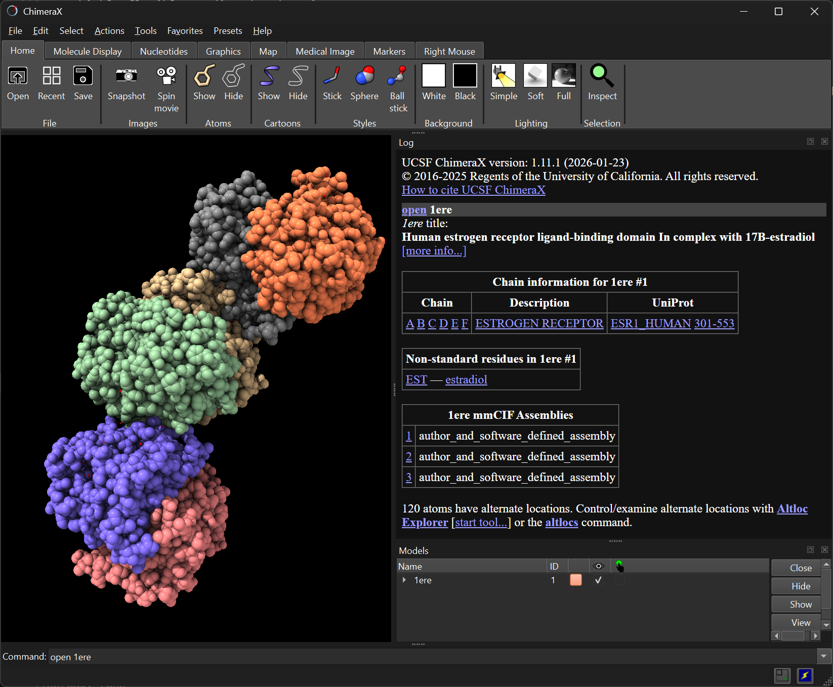
To open a PDB file from the command line, use open. For example, to load the ligand-binding domain of the human Estrogen Receptor (PDB: 1ERE):

open 1ere

The structure appears in the main window. Use the mouse to rotate, zoom, and pan.

3.3 Inspecting the structure

Use the info command to obtain information about the loaded models:

info

2 models
#1, 1ere, shown
11376 atoms, 11472 bonds, 1530 residues, 6 chains (A,B,C,D,E,F)
12 missing structure
#1.1, missing structure, shown, 12 pseudobonds

• Model #1: main structure (11376 atoms, 11472 bonds, 1530 residues, 6 chains).
• Model #1.1: missing residues (represented as pseudobonds).

To get details about chains:

info polymers

ChimeraX lists residue ranges for each chain. For 1ERE, each chain has three segments (305–330, 337–461, 465–548), repeated because this PDB entry consists of three assemblies of a homodimer (so, 3 x 2 = 6 chains).

To view metadata such as ligands:

log metadata

	Metadata for 1ere#1
Title	Human estrogen receptor ligand-binding domain In complex with 17Β-estradiol
Citation	Brzozowski, A.M., Pike, A.C., Dauter, Z., Hubbard, R.E., Bonn, T., Engstrom, O., Ohman, L., Greene, G.L., Gustafsson, J.A., Carlquist, M. (1997). Molecular basis of agonism and antagonism in the oestrogen receptor. Nature, 389, 753-758. PMID: 9338790. DOI: 10.1038/39645
Non-standard residue	EST — estradiol
Gene source	Homo sapiens (human)
Experimental method	X-ray diffraction
Resolution	3.1Å

For example, this shows the presence of residues named EST, corresponding to the Estradiol ligand included with this structure.

To list chains and their UniProt references:

log chains

Chain	Description	UniProt
A–F	Estrogen Receptor	ESR1_HUMAN 301–553

3.4 Selecting items

Selections are central in ChimeraX, and can be used to highlight, manipulate, or modify specific parts. Selections are highlighted in the viewer and can be modified or combined.

Selections use a target specifier syntax (docs), including:

• # → model number
• / → chain ID (uppercase letters)
• : → residue numbers
• @ → atom names

Examples:

• Select model #1:

  select #1

• Select chain A:

  select /A

• Select residue 500 in chain A:

  select /A:500

• Select alpha carbon of residue 305:

  select /A:305@CA

• Select residues 400–500 in chain A:

  select /A:400-500

• Clear selection:

  select clear

• Select all:

  select all

3.4.1 Combining and modifying selections

Selections can be built incrementally with select add and select subtract. Examples:

• Select all residues in chain A except for residues 400 to 500:

  select /A
  select subtract /A:400-500

• Add back residues 400 to 410:

  select add /A:400-410

Selections can be combined using logical operators:

• & (AND)
• | (OR)

Examples:

• Select residues 305–330 in either chain A or chain F:

  select /A:305-330 | /F:305-330

• Select all serine (SER) residues in a range:

  select /A:305-330 & :SER

In the last example, note how we used the aminoacid name (SER) instead of the residue number to select all serine residues in that range.

3.4.2 Select keywords

There are convenience keywords that can be used to select common groups of atoms:

Keyword	What it selects
protein	all protein atoms
nucleic	all DNA/RNA atoms
ligand	non-polymer atoms (small molecules, ions)
solvent	water molecules
sel	currently selected elements

Residues are also annotated with names. We’ve already seen how we can select all serine residues by their name using :SER.

Ligands are usually also named. For example, in our structure, the ligand (estradiol) is annotated with the keyword EST, so we can select it with:

select :EST

Alternatively, we could use the generic keyword:

select ligand

The latter would select every ligand in the loaded structures, so if there was more than one ligand, all of them would be selected this way.

Zooming and rotation

Zoom to a selection with view:

select /A:305@CA
view sel

Set the centre of rotation on a certain item with cofr. For example, set the centre of rotation on the ligand:

cofr :EST

3.5 Delete objects

You can use the delete command to remove parts of your struture from view. In our example, the 1ERE structure contains 6 repeated chains (A-F). To only keep chain A and delete the rest:

select #1/A
delete atoms ~sel

• First select chain A (/A) from the main model (#1).
• Then delete everything that is not selected: ~sel (the ~ symbol negates the selection).

The same could have been achieved with:

delete #1/B-F

3.6 Naming and saving selections

Selections can be saved for reuse.

For example, we save a selection of residues that are commonly mutated in cancers (Fuqua, Gu & Rechoum, 2015):

select /A:536,537,538
name frozen muts /A:536,537,538

Now you can refer to muts:

# zoom-in on this selection
view muts

# select these residues
select muts

# select everything except these residues
select ~muts

# colour these residues red
color muts red

3.7 Sequence viewer

Open a sequence window to visualise and select residues:

sequence chain /A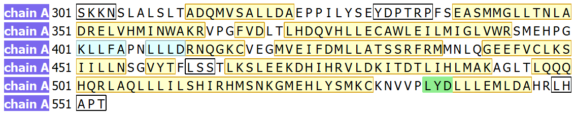

• Click residues in the sequence to select them in 3D.

• Selected residues are highlighted in green.

• Secondary structure is colour-coded: α-helix (yellow), β-strand (blue).

• Missing residues appear in black boxes.

• Residue numbers correspond to the UniProt numbering.

• Selected residues are highlighted in green.

• Secondary structure is colour-coded: β-strand in blue and α-helix in yellow.

• Missing residues appear in black boxes. These often correspond to disordered regions or flexible termini that could not be resolved in the protein structure.

3.8 Structural representations

Proteins can be represented visually in different ways.

• Cartoon representation highlights secondary structure:

  hide atoms
  show cartoon

• Atomic representation shows all atoms:

  hide cartoon
  show atoms

• Alternate atomic styles can be used:

  hide cartoon
  show atoms
  style stick
  style sphere
  style ball

• Mix representations can be used. For example, cartoon for protein, spheres for ligand:

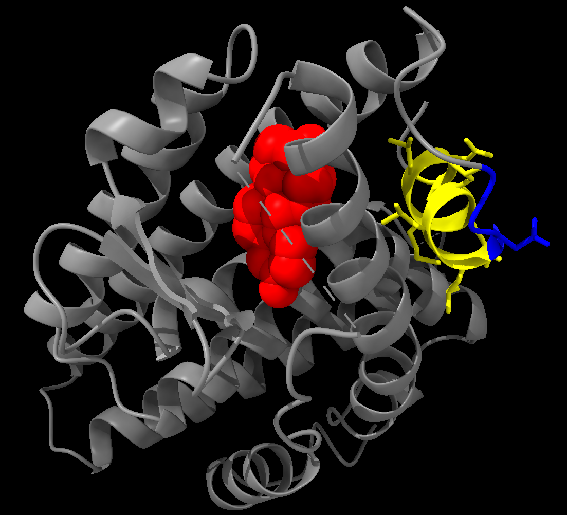
  hide atoms
  show cartoon
  show :EST
  style :EST sphere

• Colouring example:

  color protein grey
  color :538-546 yellow
  show :538-546 atoms
  style :538-546 stick
  color muts blue
  color :EST red

  • Colour the protein grey.
  • Colour residues 538-546 yellow, and show their atoms using a stick style.
  • Colour the muts selection blue.
  • Colour the ligand (EST) red.

Example representation of the 1ERE structure: protein secondary structure shown as cartoon; EST ligand shown in red with sphere-stype atoms; residues 538-546 highlighted in yellow with stick-style atoms; mutations of interest in blue with stick-style atoms.

3.9 Surface representation

You can also represent structures using surfaces, which can help visualise the shape of the molecule.

Example:

surface protein color white transparency 80

This command creates a surface representation of the protein, coloured white with 80% transparency. We keep the cartoon representation, allowing us to view the secondary structure inside the surface.

To hide the surface:

surface hide

3.10 Adding UniProt annotations

Structural information is often easier to interpret alongside functional annotations. ChimeraX can retrieve UniProt annotations directly.

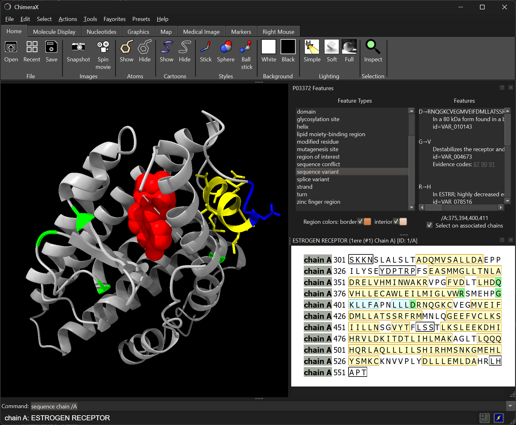
For ESR1, the corresponding UniProt entry is P03372. We can open its annotations with:

open P03372 from uniprot format uniprot

This opens a sequence annotation panel showing features such as:

• functional domains
• transmembrane regions
• experimentally observed variants
• binding sites

Clicking a feature in the panel will highlight the corresponding residues in the structure.

Combining structural and functional annotations helps identify regions likely to be sensitive to mutation.

ChimeraX snapshot of 1ERE structure with UniProt annotations panel shown on the right. In this example, we have selected “sequence variants”, which become highlighted in green in the structure, as well as the sequence viewer (bottom-right)

3.11 Saving sessions and structures

Save a ChimeraX session by changing to the destination directory, and use the save command:

cd ~/Course_Materials/
save 1ERE_annotated.cxs

.cxs is a ChimeraX-specific format. To reopen the session:

cd ~/Course_Materials/
open 1ERE_annotated.cxs

The save command can also be used to save protein structures in standard formats:

save 1ERE_annotated.pdb
save 1ERE_annotated.cif

This allows using ChimeraX to convert between struture formats: open a .pdb file and save as .cif, or vice-versa.

3.12 Exercises

ExerciseExercise 1 - Selection commands

Start a new session with the 1ERE structure (Human estrogen receptor):

close
open 1ere

Write the select commands to achieve the following:

1. Select all residues from either chain A or chain B.
2. Select everything except chain E.
3. Select all the CA atoms (alpha carbon) on residues 315-350 of chain C.

AnswerAnswer

1. We can use the OR (|) operator to select the residues in either of those chains:

   select /A | /B

2. We can use the select all command to select everything, and then subtract chain E:

   select all
   select subtract /E

3. To select atoms we can use the @ selector after the residue number:

   select /C:315-350 & @CA
   view sel

ExerciseExercise 2 - Styles and colouring

Start a new session with chain A of 1ERE (Human estrogen receptor):

close
open 1ere
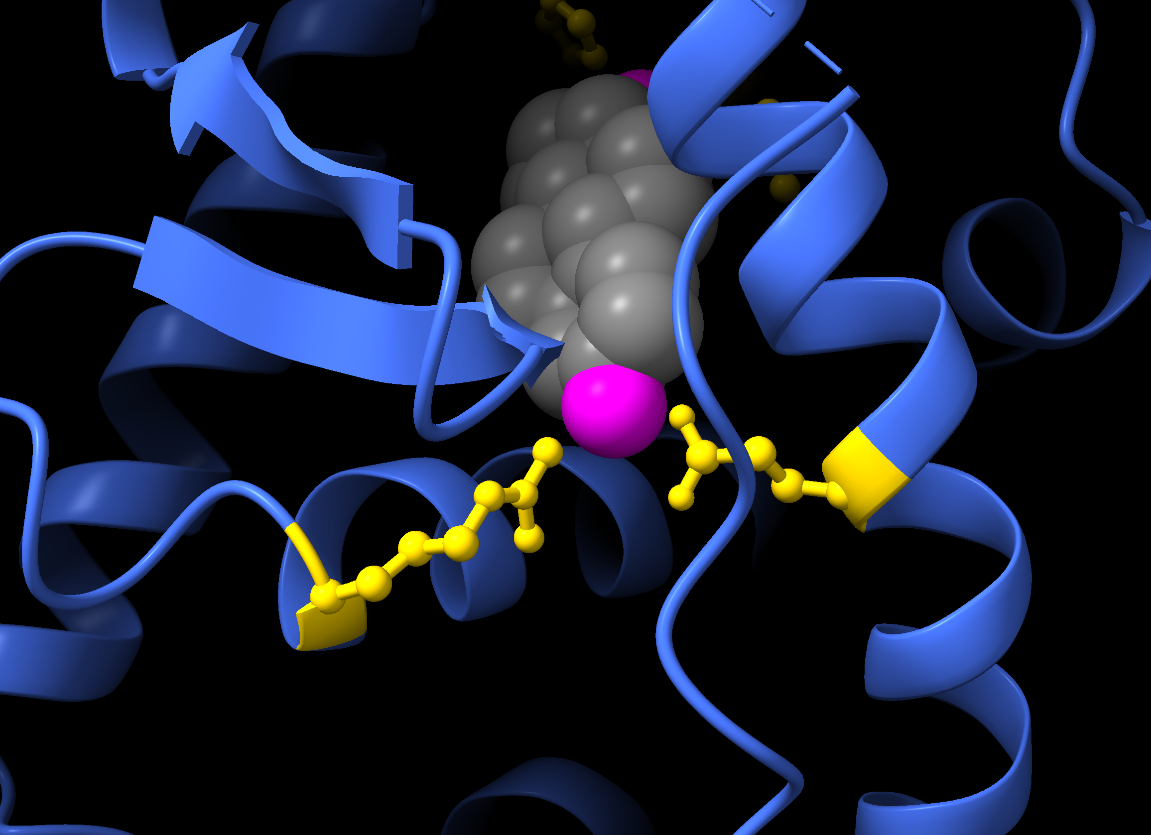
delete #1/B-F

Try to recreate the visualisation shown below, where:

• The protein is shown in cartoon representation using royalblue colour.
• The ligand (EST) is shown in sphere style using grey colour for carbon atoms and magenta for oxygen atoms.
• The key protein residues for binding the ligand - Glu353, Arg394, His524, Leu525 - are highlighted in gold colour and their atoms are shown in ball style.
• Zoom in specifically on these four residues using the view command.

Ligand view of 1ERE structure.

AnswerAnswer

Here are the steps to recreate this visualisation:

hide atoms
show cartoon
color protein royalblue
show :EST atoms
style :EST sphere
color :EST & C grey
color :EST & O magenta
show :353,394,524,525 atoms
style :353,394,524,525 ball
color :353,394,524,525 gold
view :353,394,524,525

ExerciseExercise 3 - Using UniProt annotations

Starting from this view of chain A of 1ERE:

close
open 1ere
delete #1/B-F
hide atoms
show cartoon
show :EST atoms
style :EST sphere
color :EST red

Tasks:

1. Import the UniProt annotations for ESR1 (P03372).
2. Identify which residues are annotated as ligand-binding residues.
3. Save this selection as binding_site, for later reuse.
4. Highlight these residues using a different colour, with atoms shown in ball style.
5. Can you identify a sequence variant that coincides with a ligand-binding residue? Highlight it in a different colour.

AnswerAnswer

1. We can import the UniProt annotations with:

   open P03372 from uniprot format uniprot

2. The ligand-binding residues are annotated in the sequence annotation panel as “Binding site”. In the log window we can see this corresponds to:

   select /A:353,394,524

3. We can save this selection as binding_site:

   name frozen binding_site /A:353,394,524

4. Finally, we can highlight these residues with a different colour and style:

   color binding_site gold
   show binding_site atoms
   style binding_site ball

5. By clicking through the variants listed under the “sequence variant” feature type, we can identify that residue 394 (Arg394) is annotated as a variant site. We can select this residue and highlight it in a different colour:

   select /A:394
   color sel cyan

ExerciseExercise 4 - Cartoon view and colour by chain

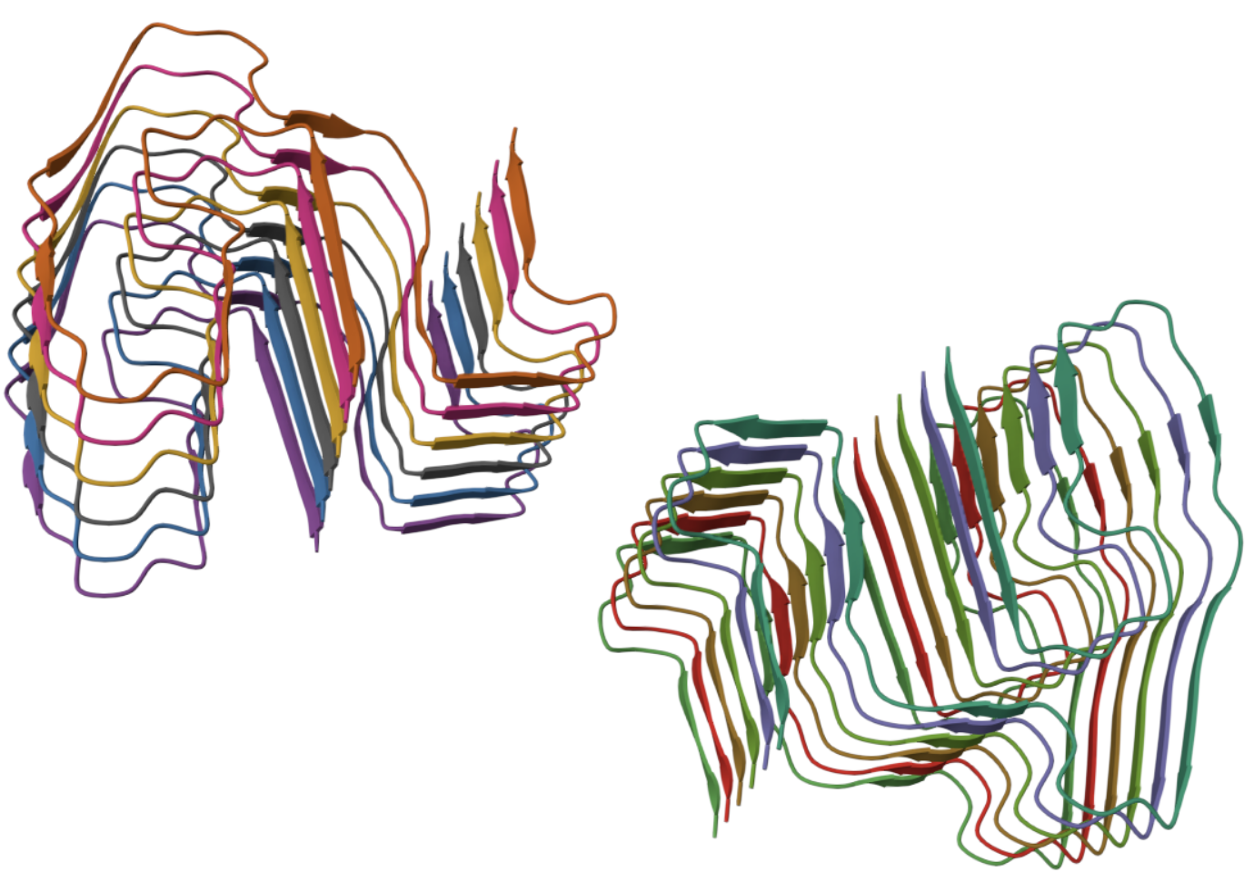
Try to recreate this view of the murine AA amyloid fibril (PDB: 6DSO):

Mus musculus AA amyloid fibril.

AnswerAnswer

This gets us close:

close 
open 6DSO
hide atoms
show cartoon
color bychain

The default colour palette doesn’t exactly match the colours shown in the image, but we could change the colours of each chain manually if desired.

ExerciseExercise 5 - Surface representation

Try and recreate this RCSB-PDB molecule of month view (PDB: 1AOI):

Complex between the Xenopus’ nucleosome (purple) with DNA (orange) wrapped around it. Image source: RCSB PDB Molecule of the Month: Nucleosome

Make sure to colour each DNA chain slightly differently. You can use log chains to find out which chains correspond to the protein and which are the DNA.

AnswerAnswer

This gets us close to the visualisation:

close
open 1AOI
surface protein
surface nucleic
colour protein plum
colour /I tomato
colour /J coral

We used log chains to find out that chains I and J correspond to the DNA, and coloured them differently using the colour command.

ExerciseExercise 6 - Surfaces and annotations

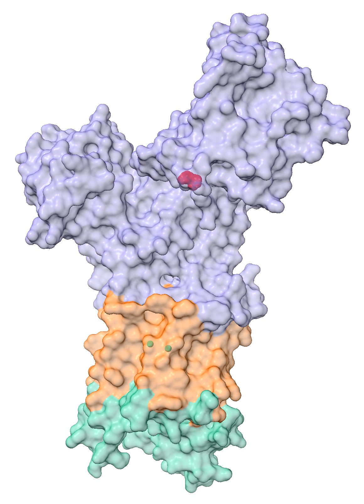
Try to create a similar view to the following RBSB-PDB molecule of the month (PDB: 1SU4).

ATP-driven calcium pump in the sarcoplasmic reticulum membrane that restores low cytosolic calcium to enable muscle relaxation. Image source: RCSB PDB Molecule of the Month: Calcium Pump

It might be hard to recreate exactly the same view, but here are some guidelines for what you could try:

• Hide the atoms
• Draw a surface representation of the protein using a transparency of 60%
• Show the calcium ion and colour it cyan
  • Use log metadata to see how the Calcium molecule is called
• Import metadata from UniProt (you might have to go to PDB to find the UniProt ID). This should allow you to select:
  • Active site: Show as atoms and colour red
  • Topological domain lumenal: Colour #1b9e77
  • topological domain cytoplasmic: Colour #7570b3
  • transmembrane region: Colour #d95f02

AnswerAnswer

We start by opening the structure and hiding the atoms, then showing the surface representation of the protein with a transparency of 60%, and showing the CA atoms coloured cyan:

close
open 1SU4
hide cartoon
hide atoms
surface protein transparency 60
show :CA
colour :CA cyan

We import metadata from UniProt, using the UniProt ID P04191, which we can find in the PDB entry for 1SU4:

open P04191 from uniprot format uniprot

We select each of the features indicated, and colour them accordingly. Here, we give the exact residues, which we copied from the log window, as we clicked on each of the UniProt annotations.

select /A:70-89,274-295,778-787,852-897,950-964
colour sel #1b9e77
select /A:1-48,111-253,314-757,809-828,918-930,986-994
colour sel #7570b3
select /A:49-69,90-110,254-273,296-313,758-777,788-808,829-851,898-917,931-949,965-985
colour sel #d95f02
select /A:351
show sel atoms
style sel sphere
colour sel red
select clear

This should give you the following view:

3.13 Summary

TipKey points

At first, ChimeraX may look like a graphics program, however its real power comes from its range of commands and flexible selection syntax.

• ChimeraX combines a graphical interface and command line interface.

• Structures are loaded with the open command. ChimeraX can fetch structures directly from the PDB using their identifier.

• Structural information can be inspected using info commands. These commands reveal models, chains, residues, ligands, and experimental metadata.

• ChimeraX uses a concise syntax to specify models (#), chains (/), residues (:), and atoms (@).

• Selections can be modified and combined. Commands such as add, subtract, &, and | allow complex selections.

• Structures can be displayed in different representations:

  • Cartoon views emphasise secondary structure
  • Atom-based views show detailed interactions
  • Surface views reveal overall shape and interfaces

• Saving selections allows you to refer to important residues or regions later.

• ChimeraX sessions can be saved and reopened. This allows you to preserve visualisations and annotations for later work.

ChimeraX documentation

• ChimeraX User Guide https://www.cgl.ucsf.edu/chimerax/docs/user/index.html

• ChimeraX Tutorials https://www.cgl.ucsf.edu/chimerax/tutorials.html