gapminder <- read_csv("data/gapminder_clean.csv")13 Making data stand out
Learning outcomes
- Learn how to make some data stand out from the crowd
13.1 Libraries and functions
Click to expand
13.1.1 Libraries
13.1.2 Functions
13.2 Purpose and aim
Often we have to deal with large amounts of data. But even more often we want to draw the reader’s attention to a particular property of the data that we’re displaying. In these cases it can be useful to visually let your data stand out.
13.3 Loading data
If you haven’t done so yet, please load the data as follows:
13.4 The popout
To be honest, I’m not entirely sure if this is a word, but it’s a technique that is often used in visualisation. Here we’re colouring our data of interest in a highly contrasting way to the rest of the data, to make them “pop out”.
Have a look at the following plot, where we are plotting child mortality against the number of children per woman:
ggplot(data = gapminder,
       aes(x = children_per_woman,
           y = child_mortality)) +
  geom_point()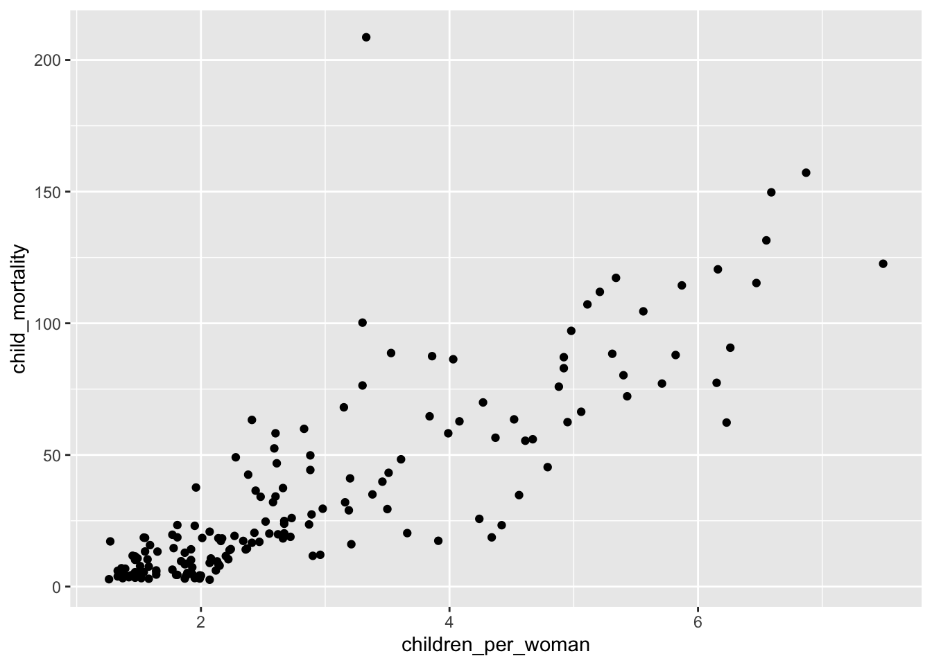
It looks like there is a strong positive correlation between the number of children per women and child mortality, since child mortality seems to increase as the number of children per woman is higher.
In our data set we have a variable called is_oecd, which contains TRUE/FALSE statements on whether a country is part of the Organisation for Economic Co-operation and Development. This organisation stimulates economic progress and world trade and consists of primarily richer, Western countries.
Let’s say we wanted to explore if this possible correlation has something to do with the economic status of the country. If that’s the case, it could be that child mortality rates in OECD countries is perhaps not linked to the number of children per women, whereas it is in non-OECD countries. Perhaps differences in the quality of healthcare lead to better survival rates for children in richer countries, even if a woman has many children.
We can visualise this.
ggplot(data = gapminder,
       aes(x = children_per_woman,
           y = child_mortality,
           colour = is_oecd)) +
  geom_point()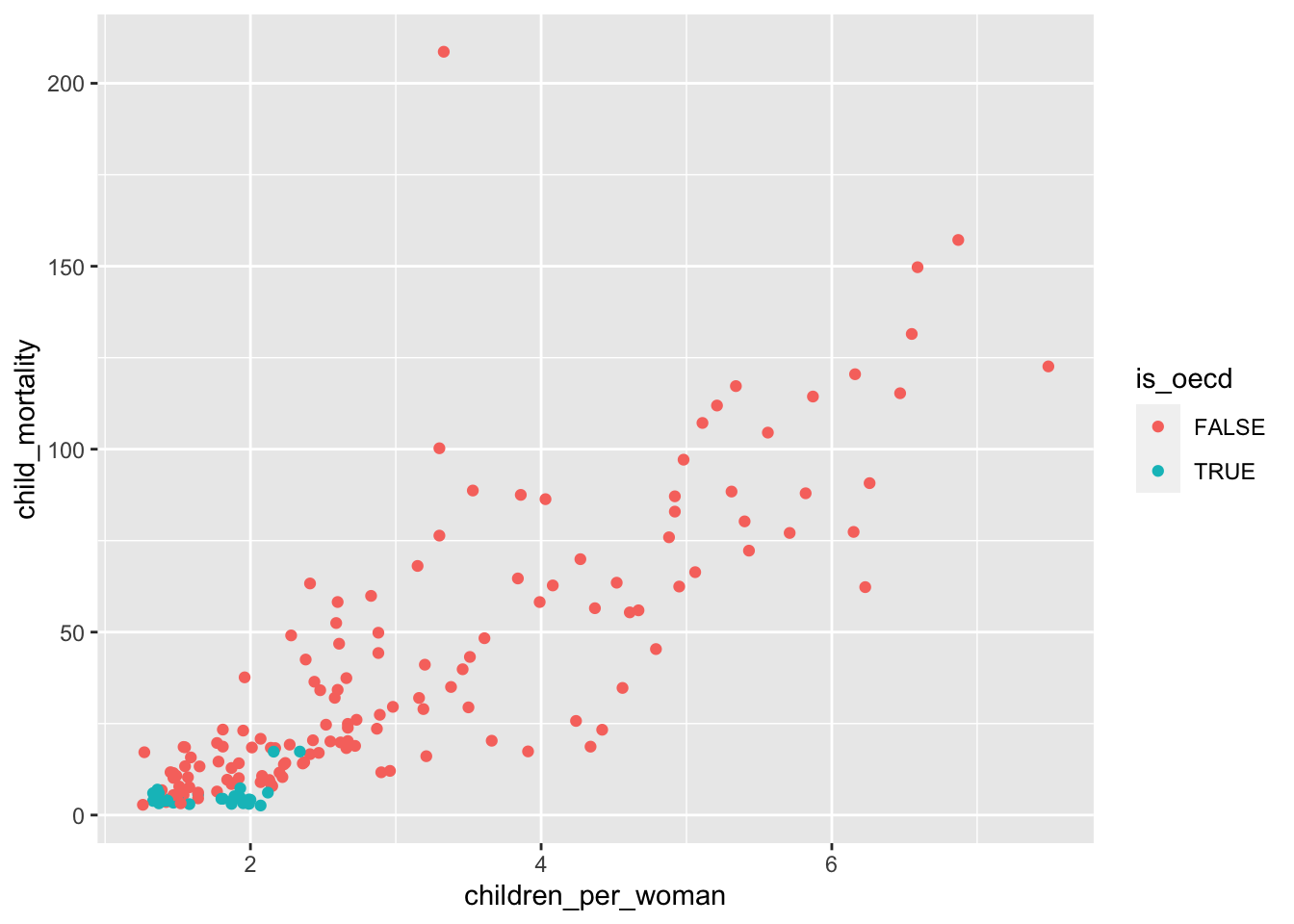
It looks like child mortality rates in non-OECD countries are much more variable than in OECD countries. There doesn’t appear to be enough spread in the OECD country data to draw conclusions about the OECD countries.
We’ve previously seen that life expectancy is poor in sub-Saharan Africa. It would therefore be interesting to investigate if that has anything to do with high levels of child mortality.
To visualise this we need to colour the data of the sub-Saharan Africa world_region a different colour than the rest of the data.
We can use a similar technique as we did for the OECD countries. We first need to create a column that contains information about whether a country is in sub-Saharan Africa and then colour the data accordingly.
Here we also manually update the colours to increase data discriminability.
gapminder %>%
  mutate(is_sub_saharan_africa = world_region == "sub_saharan_africa") %>%
  ggplot(aes(x = children_per_woman,
             y = child_mortality,
             colour = is_sub_saharan_africa)) +
  geom_point() +
  scale_colour_manual(values = c("grey", "firebrick"))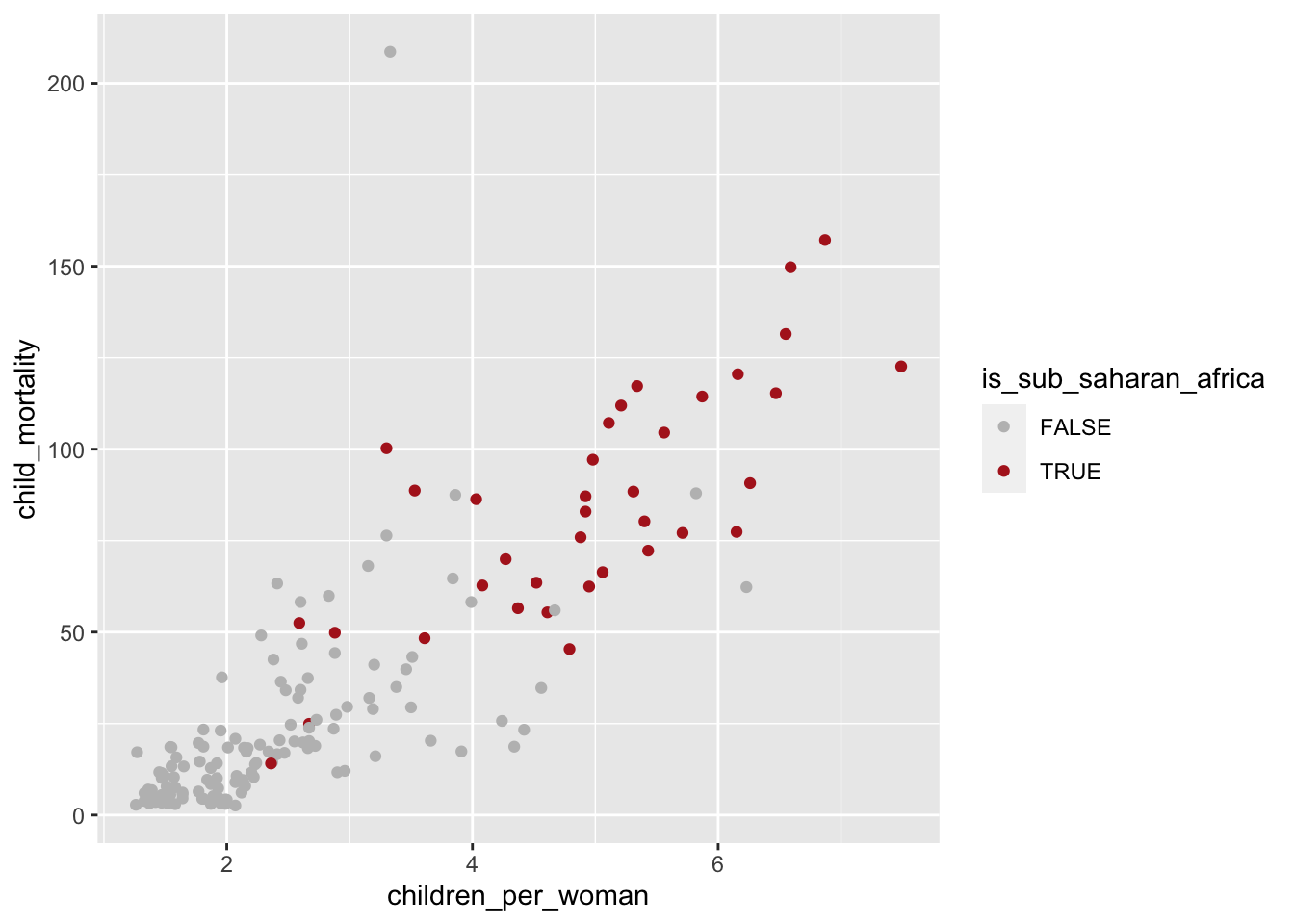
13.4.1 Exercises
Income vs life expectancy in South Asia
Level:
Plot income (x-axis) against life expectancy for women (y-axis), colouring the data for South Asia differently from the rest of the data. Ensure that there is sufficient contrast between the two groups of data points.
Answer
gapminder %>%
  mutate(is_south_asia = world_region == "south_asia") %>%
  ggplot(aes(x = income_per_person,
         y = life_expectancy_female,
         colour = is_south_asia)) +
  geom_point() +
  scale_colour_manual(values = c("grey", "firebrick"))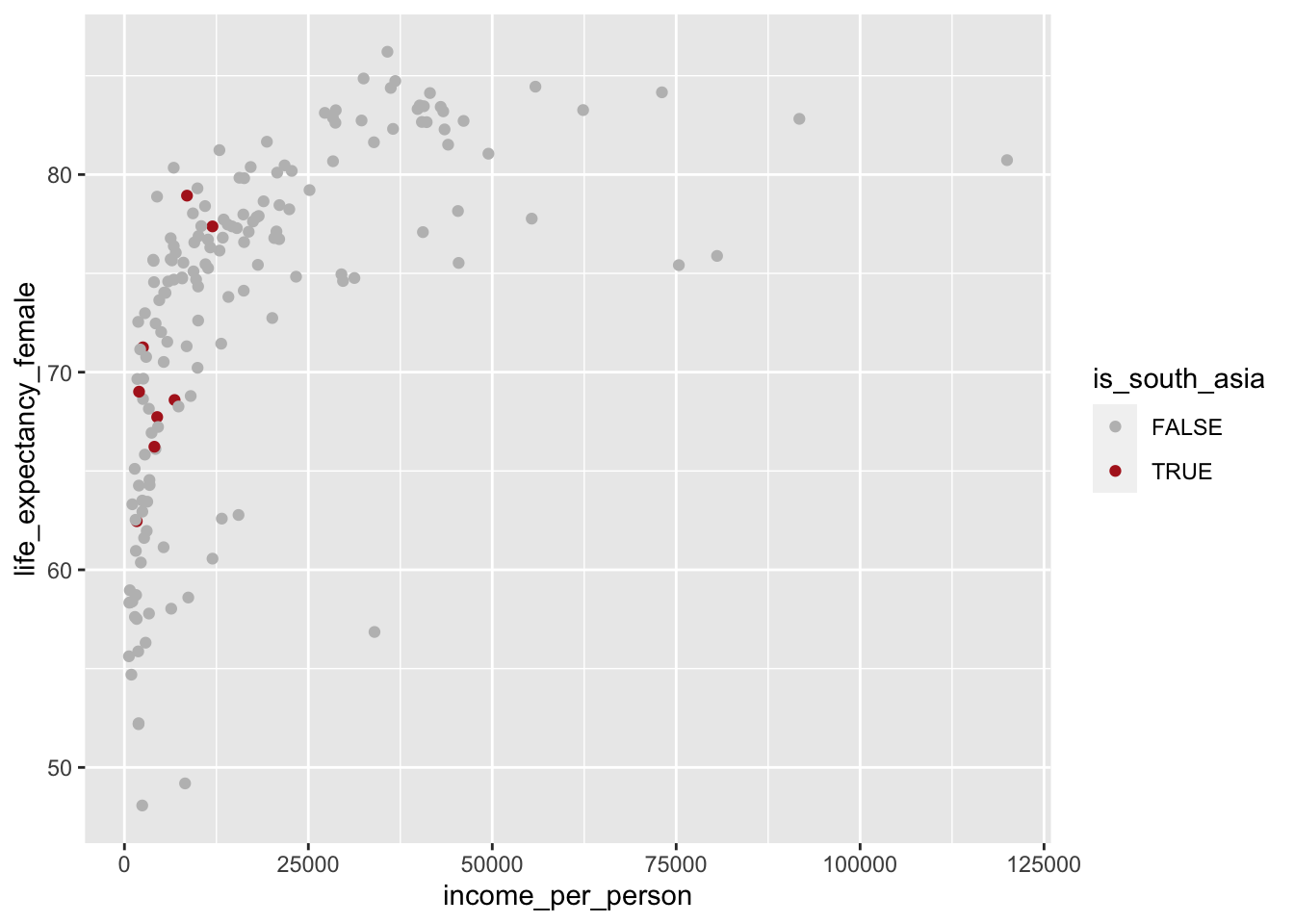
Ordering and emphasising groups
Level:
Create a bar plot that contains the income per person, split by world region.
Ensure that the data is arranged in ascending order (based on average income across each region) and highlight East-Asia Pacific.
Answer
We’re combining some skills from the ordering/ranking section with the popout.
First we need to find the average income for each region, and then colour East-Asia Pacific. To colour the inside of the bar plot we need to use the fill instead of the colour argument (see what happens if you do use colour!).
gapminder %>%
  group_by(world_region) %>%
  summarise(mean_income = mean(income_per_person)) %>%
  ungroup() %>%
  mutate(is_eap = world_region == "east_asia_pacific") %>%
  ggplot(aes(x = fct_reorder(world_region, mean_income),
             y = mean_income,
             fill = is_eap)) +
  geom_bar(stat = "identity") +
  theme(axis.text.x = element_text(angle = 45, hjust=1)) +
  labs(x = "World region", y = "Mean income")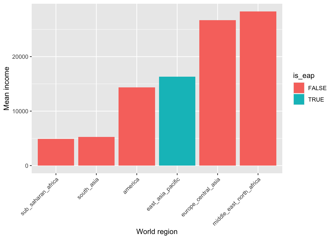
13.5 Summary
Key points
- We can use a popout to emphasise data