library(broom)
library(tidyverse)
library(performance)

# You will likely need to install this package first
library(lmtest)9 Significance testing
Learning outcomes
- Understand the concept of statistical deviance
- Use likelihood ratio tests to perform significance testing for:
- An entire model (versus the null model)
- Individual predictor variables
9.1 Libraries and functions
Click to expand
import math
import pandas as pd
from plotnine import *
import statsmodels.api as sm
import statsmodels.formula.api as smf
from scipy.stats import *
import numpy as np
Generalised linear models are fitted a little differently to standard linear models - namely, using maximum likelihood estimation instead of ordinary least squares for estimating the model coefficients.
As a result, we can no longer use F-tests for significance, or interpret \(R^2\) values in quite the same way. This section will introduce likelihood ratio tests, a method for extracting p-values for GLMs.
9.2 Deviance
Several of the tests and metrics we’ll discuss below are based heavily on deviance. So, what is deviance, and where does it come from?
Here’s a few key definitions:
| Maximum likelihood estimation | This is the method by which we fit the GLM (i.e., find the values for the beta coefficients). As the name suggests, we are trying to find the beta coefficients that maximise the likelihood of the dataset/sample. |
| Likelihood | In this context, “likelihood” refers to the joint probability of all of the data points in the sample. In other words, how likely is it that you would sample a set of data points like these, if they were being drawn from an underlying population where your model is true? Each candidate model fitted to a dataset will have its own unique likelihood. |
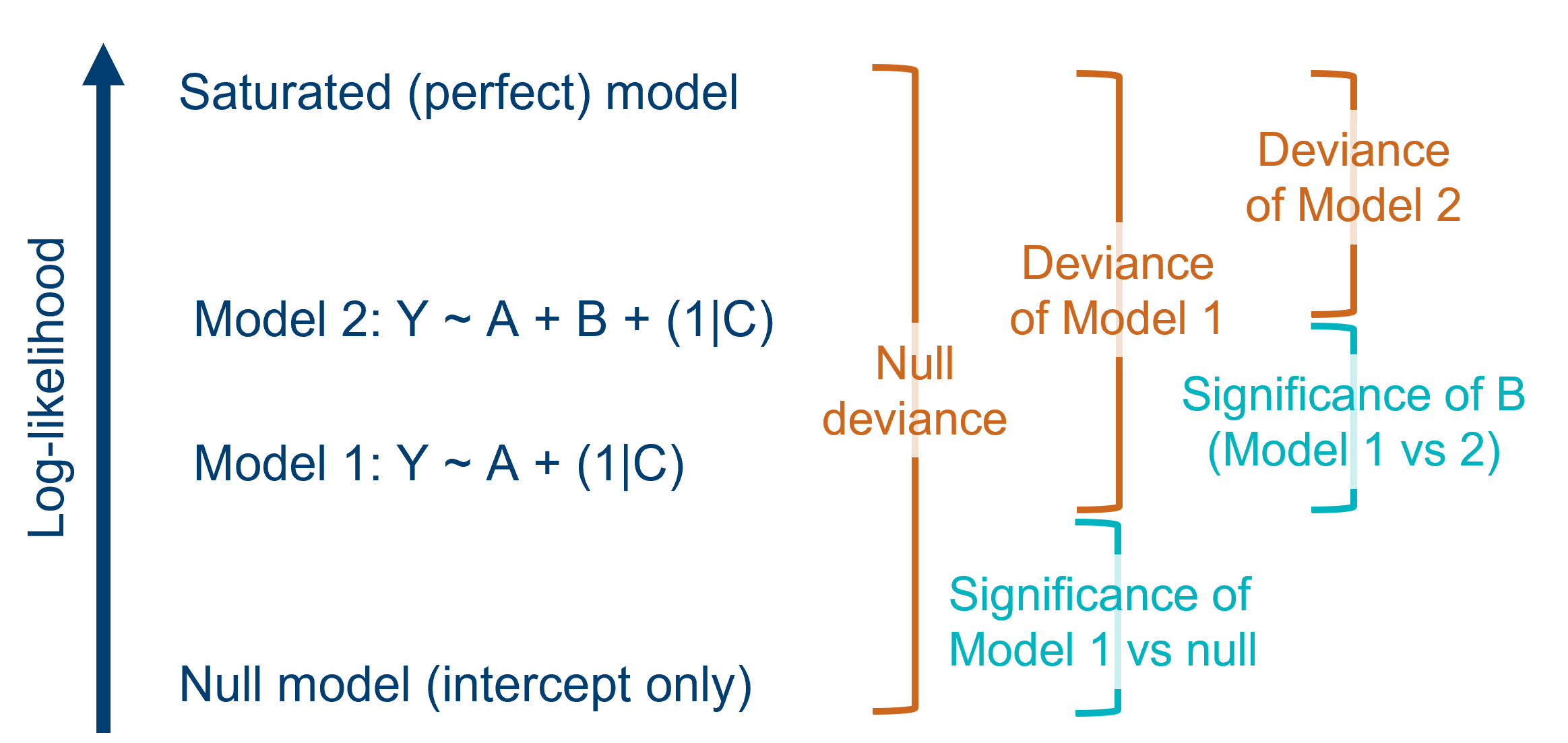
| Saturated (perfect) model | For each dataset, there is a “saturated”, or perfect, model. This model has the same number of parameters in it as there are data points, meaning the data are fitted exactly - as if connecting the dots between them. This model has the largest possible likelihood of any model fitted to the dataset. Of course, we don’t actually use the saturated model for drawing real conclusions, but we can use it as a baseline for comparison. |
| Deviance (residual deviance) |
Each candidate model is compared back to the saturated model to figure out its deviance. Deviance is defined as the difference between the log-likelihood of your fitted model and the log-likelihood of the saturated model (multiplied by 2). Because deviance is all about capturing the discrepancy between fitted and actual values, it’s performing a similar function to the residual sum of squares (RSS) in a standard linear model. In fact, the RSS is really just a specific type of deviance. Sometimes, the deviance of a candidate (non-null) model is referred to more fully as “residual deviance”. |
| Null deviance | One of the models that we can compare against the saturated model is the null model (a model with no predictors). This gives us the deviance value for the null model. This is the greatest deviance of any possible model that could be fitted to the data, because it explains zero variance in the response variable. |
9.3 Revisiting the diabetes dataset
As a worked example, we’ll use a logistic regression fitted to the diabetes dataset that we saw in a previous section.
diabetes <- read_csv("data/diabetes.csv")Rows: 728 Columns: 3
── Column specification ────────────────────────────────────────────────────────
Delimiter: ","
dbl (3): glucose, diastolic, test_result
ℹ Use `spec()` to retrieve the full column specification for this data.
ℹ Specify the column types or set `show_col_types = FALSE` to quiet this message.diabetes_py = pd.read_csv("data/diabetes.csv")
diabetes_py.head() glucose diastolic test_result
0 148 72 1
1 85 66 0
2 183 64 1
3 89 66 0
4 137 40 1As a reminder, this dataset contains three variables:
test_result, binary results of a diabetes test result (1 for positive, 0 for negative)glucose, the results of a glucose tolerance testdiastolicblood pressure
glm_dia <- glm(test_result ~ glucose * diastolic,
                  family = "binomial",
                  data = diabetes)
model = smf.glm(formula = "test_result ~ glucose * diastolic",
family = sm.families.Binomial(),
data = diabetes_py)
glm_dia_py = model.fit()9.4 What are the p-values in the summary?
You might have noticed that when you use summary to see the model output, it comes with some p-values automatically.
What are they? Can you use/interpret them?
summary(glm_dia)
Call:
glm(formula = test_result ~ glucose * diastolic, family = "binomial",
data = diabetes)
Coefficients:
Estimate Std. Error z value Pr(>|z|)
(Intercept) -8.5710565 2.7032318 -3.171 0.00152 **
glucose 0.0547050 0.0209256 2.614 0.00894 **
diastolic 0.0423651 0.0363681 1.165 0.24406
glucose:diastolic -0.0002221 0.0002790 -0.796 0.42590
---
Signif. codes: 0 '***' 0.001 '**' 0.01 '*' 0.05 '.' 0.1 ' ' 1
(Dispersion parameter for binomial family taken to be 1)
Null deviance: 936.60 on 727 degrees of freedom
Residual deviance: 748.01 on 724 degrees of freedom
AIC: 756.01
Number of Fisher Scoring iterations: 4print(glm_dia_py.summary()) Generalized Linear Model Regression Results
==============================================================================
Dep. Variable: test_result No. Observations: 728
Model: GLM Df Residuals: 724
Model Family: Binomial Df Model: 3
Link Function: Logit Scale: 1.0000
Method: IRLS Log-Likelihood: -374.00
Date: Wed, 09 Jul 2025 Deviance: 748.01
Time: 16:43:31 Pearson chi2: 720.
No. Iterations: 5 Pseudo R-squ. (CS): 0.2282
Covariance Type: nonrobust
=====================================================================================
coef std err z P>|z| [0.025 0.975]
-------------------------------------------------------------------------------------
Intercept -8.5711 2.703 -3.171 0.002 -13.869 -3.273
glucose 0.0547 0.021 2.614 0.009 0.014 0.096
diastolic 0.0424 0.036 1.165 0.244 -0.029 0.114
glucose:diastolic -0.0002 0.000 -0.796 0.426 -0.001 0.000
=====================================================================================Each individual parameter, or coefficient, has its own z-value and associated p-value. In each case, a hypothesis test has been performed - these are formally called Wald tests.
The null hypothesis for these Wald tests is that the value of the coefficient = 0. The idea is that if a coefficient isn’t significantly different from 0, then that parameter isn’t useful and could be dropped from the model.
These tests are the equivalent of the t-tests that are calculated as part of the summary output for standard linear models.
Why can’t we just use these p-values?
In some cases, you can. However, there are a few cases where they don’t give you all the info you need.
Firstly: they don’t tell you about the significance of the model as a whole (versus the null model).
Secondly: for categorical predictors, you will get a separate Wald p-value for each non-reference group (compared back to the reference group). This is not the same as a p-value for the categorical predictor as a whole. The Wald p-values can also be heavily affected by which group was chosen as the reference.
It’s typically preferable to use a likelihood ratio test instead.
9.5 Likelihood ratio tests (LRTs)
When we were assessing the significance of standard linear models, we were able to use the F-statistic to determine:
- the significance of the model versus a null model, and
- the significance of individual predictors.
We can’t use these F-tests for GLMs, but we can use LRTs in a really similar way, to calculate p-values for both the model as a whole, and for individual variables.
These tests are all built on the idea of deviance, or the likelihood ratio, as discussed above on this page. We can compare any two models fitted to the same dataset by looking at the difference in their deviances, also known as the difference in their log-likelihoods, or more simply as a likelihood ratio.
Helpfully, this likelihood ratio approximately follows a chi-square distribution, which we can capitalise on to calculate a p-value. All we need is the number of degrees of freedom, which is equal to the difference in the number of parameters of the two models you’re comparing.
Warning
Importantly, we are only able to use this sort of test when one of the two models that we are comparing is a “simpler” version of the other, i.e., one model has a subset of the parameters of the other model.
So while we could perform an LRT just fine between these two models: Y ~ A + B + C and Y ~ A + B + C + D, or between any model and the null (Y ~ 1), we would not be able to use this test to compare Y ~ A + B + C and Y ~ A + B + D.
9.5.1 Testing the model versus the null
Since LRTs involve making a comparison between two models, we must first decide which models we’re comparing, and check that one model is a “subset” of the other.
Let’s use an example from a previous section of the course, where we fitted a logistic regression to the diabetes dataset.
The first step is to create the two models that we want to compare: our original model, and the null model (with and without predictors, respectively).
glm_dia <- glm(test_result ~ glucose * diastolic,
family = "binomial",
data = diabetes)
glm_null <- glm(test_result ~ 1,
family = binomial,
data = diabetes)Then, we use the lrtest function from the lmtest package to perform the test itself; we include both the models that we want to compare, listing them one after another.
lrtest(glm_dia, glm_null)Likelihood ratio test
Model 1: test_result ~ glucose * diastolic
Model 2: test_result ~ 1
#Df LogLik Df Chisq Pr(>Chisq)
1 4 -374.0
2 1 -468.3 -3 188.59 < 2.2e-16 ***
---
Signif. codes: 0 '***' 0.001 '**' 0.01 '*' 0.05 '.' 0.1 ' ' 1We can see from the output that our chi-square statistic is significant, with a really small p-value. This tells us that, for the difference in degrees of freedom (here, that’s 3), the change in deviance is actually quite big. (In this case, you can use summary(glm_dia) to see those deviances - 936 versus 748!)
In other words, our model is better than the null.
The first step is to create the two models that we want to compare: our original model, and the null model (with and without our predictor, respectively).
model = smf.glm(formula = "test_result ~ glucose * diastolic",
                family = sm.families.Binomial(),
                data = diabetes_py)

glm_dia_py = model.fit()
model = smf.glm(formula = "test_result ~ 1",
family = sm.families.Binomial(),
data = diabetes_py)
glm_null_py = model.fit()Unlike in R, there isn’t a nice neat function for extracting the \(\chi^2\) value, so we have to do a little bit of work by hand.
# calculate the likelihood ratio (i.e. the chi-square value)
lrstat = -2*(glm_null_py.llf - glm_dia_py.llf)

# calculate the associated p-value
pvalue = chi2.sf(lrstat, glm_null_py.df_resid - glm_dia_py.df_resid)

print(lrstat, pvalue)
188.59314837444526 1.2288700360045204e-40This gives us the likelihood ratio, based on the log-likelihoods that we’ve extracted directly from the models, which approximates a chi-square distribution.
We’ve also calculated the associated p-value, by providing the difference in degrees of freedom between the two models (in this case, that’s simply 1, but for more complicated models it’s easier to extract the degrees of freedom directly from the model as we’ve done here).
Here, we have a large chi-square statistic and a small p-value. This tells us that, for the difference in degrees of freedom (here, that’s 1), the change in deviance is actually quite big. (In this case, you can use glm_dia_py.summary() to see those deviances - 936 versus 748!)
In other words, our model is better than the null.
9.5.2 Testing individual predictors
As well as testing the overall model versus the null, we might want to test particular predictors to determine whether they are individually significant.
The way to achieve this is essentially to perform a series of “targeted” likelihood ratio tests. In each LRT, we’ll compare two models that are almost identical - one with, and one without, our variable of interest in each case.
The first step is to construct a new model that doesn’t contain our predictor of interest. Let’s test the glucose:diastolic interaction.
glm_dia_add <- glm(test_result ~ glucose + diastolic,
                  family = "binomial",
                  data = diabetes)
Now, we can use the lrtest function (or the anova function) to compare the models with and without the interaction:
lrtest(glm_dia, glm_dia_add)Likelihood ratio test
Model 1: test_result ~ glucose * diastolic
Model 2: test_result ~ glucose + diastolic
#Df LogLik Df Chisq Pr(>Chisq)
1 4 -374.00
2 3 -374.32 -1 0.6288 0.4278This tells us that our interaction glucose:diastolic isn’t significant - our more complex model doesn’t have a meaningful reduction in deviance.
This might, however, seem like a slightly clunky way to test each individual predictor. Luckily, we can also use our trusty anova function with an extra argument to tell us about individual predictors.
By specifying that we want to use a chi-squared test, we are able to construct an analysis of deviance table (as opposed to an analysis of variance table) that will perform the likelihood ratio tests for us for each predictor:
anova(glm_dia, test="Chisq")Analysis of Deviance Table
Model: binomial, link: logit
Response: test_result
Terms added sequentially (first to last)
Df Deviance Resid. Df Resid. Dev Pr(>Chi)
NULL 727 936.60
glucose 1 184.401 726 752.20 < 2e-16 ***
diastolic 1 3.564 725 748.64 0.05905 .
glucose:diastolic 1 0.629 724 748.01 0.42779
---
Signif. codes: 0 '***' 0.001 '**' 0.01 '*' 0.05 '.' 0.1 ' ' 1You’ll spot that the p-values we get from the analysis of deviance table match the p-values you could calculate yourself using lrtest; this is just more efficient when you have a complex model!
The first step is to construct a new model that doesn’t contain our predictor of interest. Let’s test the glucose:diastolic interaction.
model = smf.glm(formula = "test_result ~ glucose + diastolic",
                family = sm.families.Binomial(),
                data = diabetes_py)

glm_dia_add_py = model.fit()
We’ll then use the same code we used above, to compare the models with and without the interaction:
lrstat = -2*(glm_dia_add_py.llf - glm_dia_py.llf)

pvalue = chi2.sf(lrstat, glm_dia_py.df_model - glm_dia_add_py.df_model)

print(lrstat, pvalue)
0.6288201373598667 0.4277884257680492This tells us that our interaction glucose:diastolic isn’t significant - our more complex model doesn’t have a meaningful reduction in deviance.
9.6 Exercises
9.6.1 Predicting failure
Exercise
Level:
In the previous chapter, we used the challenger.csv dataset as a worked example.
Our research question was: should NASA have cancelled the Challenger launch, based on the data they had about o-rings in previous launches?
Let’s try to come up with an interpretation from these data, with the help of a likelihood ratio test.
You should:
- Refit the model (if it’s not still in your environment from last chapter)
- Fit a null model (no predictors)
- Perform a likelihood ratio test to compare the model to the null model
- Decide what you think the answer is to the research question
Answer
Let’s read in our data and mutate it to contain the relevant variables (this is borrowed from the last chapter):
challenger <- read_csv("data/challenger.csv") %>%
  mutate(total = 6,                     # total number of o-rings
         intact = 6 - damage,           # number of undamaged o-rings
         prop_damaged = damage / total) # proportion damaged o-rings
Rows: 23 Columns: 2
── Column specification ────────────────────────────────────────────────────────
Delimiter: ","
dbl (2): temp, damage
ℹ Use `spec()` to retrieve the full column specification for this data.
ℹ Specify the column types or set `show_col_types = FALSE` to quiet this message.We create our logistic model like so:
glm_chl <- glm(cbind(damage, intact) ~ temp,
               family = binomial,
               data = challenger)
We can get the model parameters as follows:
summary(glm_chl)
Call:
glm(formula = cbind(damage, intact) ~ temp, family = binomial,
    data = challenger)

Coefficients:
            Estimate Std. Error z value Pr(>|z|)
(Intercept) 11.66299    3.29626   3.538 0.000403 ***
temp        -0.21623    0.05318  -4.066 4.78e-05 ***
---
Signif. codes:  0 '***' 0.001 '**' 0.01 '*' 0.05 '.' 0.1 ' ' 1

(Dispersion parameter for binomial family taken to be 1)

    Null deviance: 38.898  on 22  degrees of freedom
Residual deviance: 16.912  on 21  degrees of freedom
AIC: 33.675

Number of Fisher Scoring iterations: 6
And let’s visualise the model, just to make sure it looks sensible.
ggplot(challenger, aes(temp, prop_damaged)) +
  geom_point() +
  geom_smooth(method = "glm", se = FALSE, fullrange = TRUE,
              method.args = list(family = binomial)) +
  xlim(25,85)
Warning in eval(family$initialize): non-integer #successes in a binomial glm!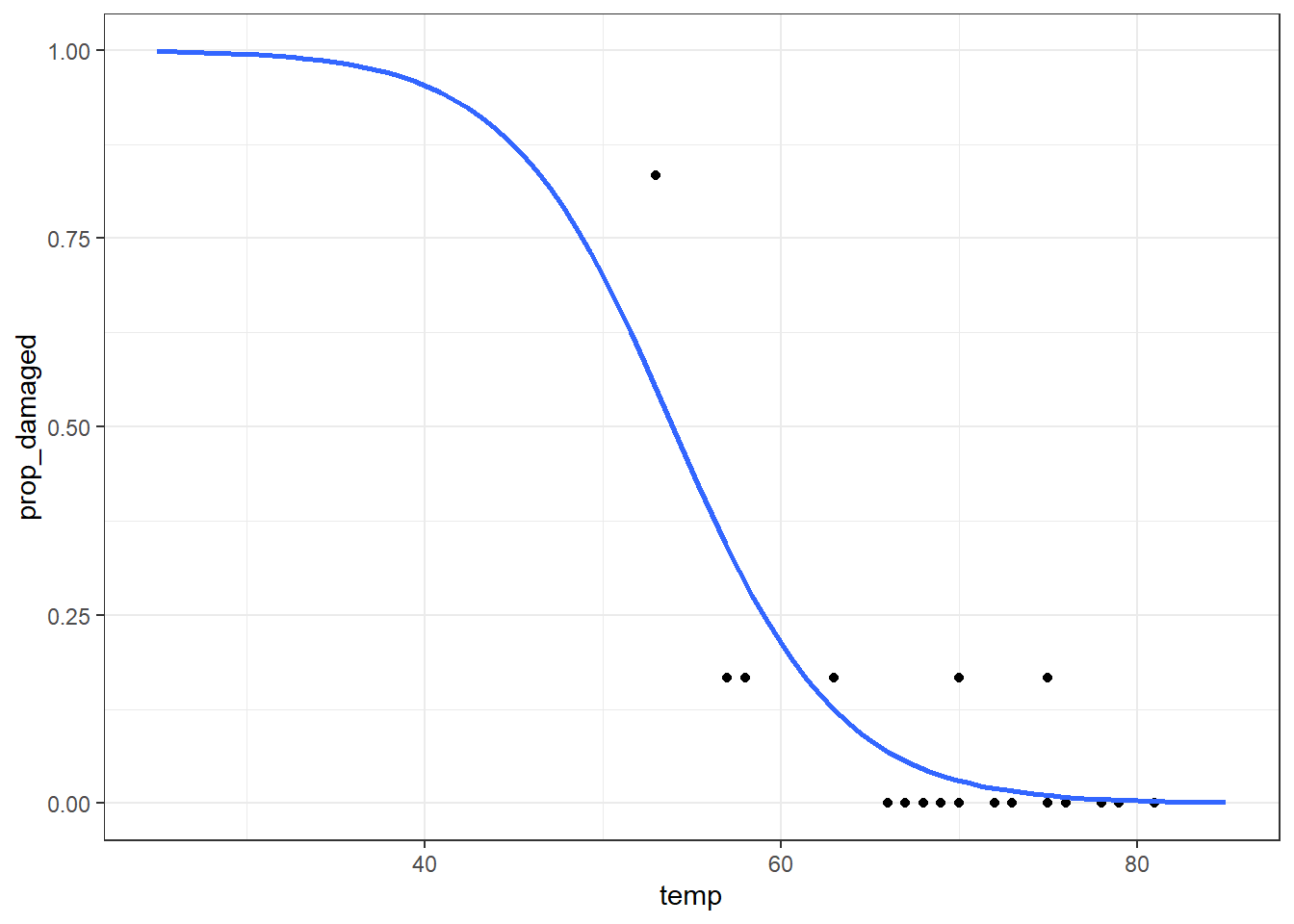
Comparing against the null
The next question we can ask is: is our model any better than the null model?
First, we define the null model; then we use lrtest to compare them.
glm_chl_null <- glm(cbind(damage, intact) ~ 1,
                family = binomial,
                data = challenger)

lrtest(glm_chl, glm_chl_null)
Likelihood ratio test
Model 1: cbind(damage, intact) ~ temp
Model 2: cbind(damage, intact) ~ 1
#Df LogLik Df Chisq Pr(>Chisq)
1 2 -14.837
2 1 -25.830 -1 21.985 2.747e-06 ***
---
Signif. codes: 0 '***' 0.001 '**' 0.01 '*' 0.05 '.' 0.1 ' ' 1With a very small p-value (and a large chi-square statistic), it would seem that the model is indeed significantly better than the null.
Since there’s only one predictor variable, this is pretty much equivalent to saying that temp does predict the proportion of o-rings that are damaged.
We need to make sure we’ve read in our data, and mutated it to contain the relevant variables (this is borrowed from the last chapter):
Our logistic regression is fitted like so:
# create a generalised linear model
model = smf.glm(formula = "damage + intact ~ temp",
                family = sm.families.Binomial(),
                data = challenger_py)
# and get the fitted parameters of the model
glm_chl_py = model.fit()
We can get the model parameters as follows:
print(glm_chl_py.summary()) Generalized Linear Model Regression Results
================================================================================
Dep. Variable: ['damage', 'intact'] No. Observations: 23
Model: GLM Df Residuals: 21
Model Family: Binomial Df Model: 1
Link Function: Logit Scale: 1.0000
Method: IRLS Log-Likelihood: -14.837
Date: Wed, 09 Jul 2025 Deviance: 16.912
Time: 16:43:33 Pearson chi2: 28.1
No. Iterations: 7 Pseudo R-squ. (CS): 0.6155
Covariance Type: nonrobust
==============================================================================
coef std err z P>|z| [0.025 0.975]
------------------------------------------------------------------------------
Intercept 11.6630 3.296 3.538 0.000 5.202 18.124
temp -0.2162 0.053 -4.066 0.000 -0.320 -0.112
==============================================================================Generate new model data:
model = pd.DataFrame({'temp': list(range(25, 86))})

model["pred"] = glm_chl_py.predict(model)

model.head()
temp pred
0 25 0.998087
1 26 0.997626
2 27 0.997055
3 28 0.996347
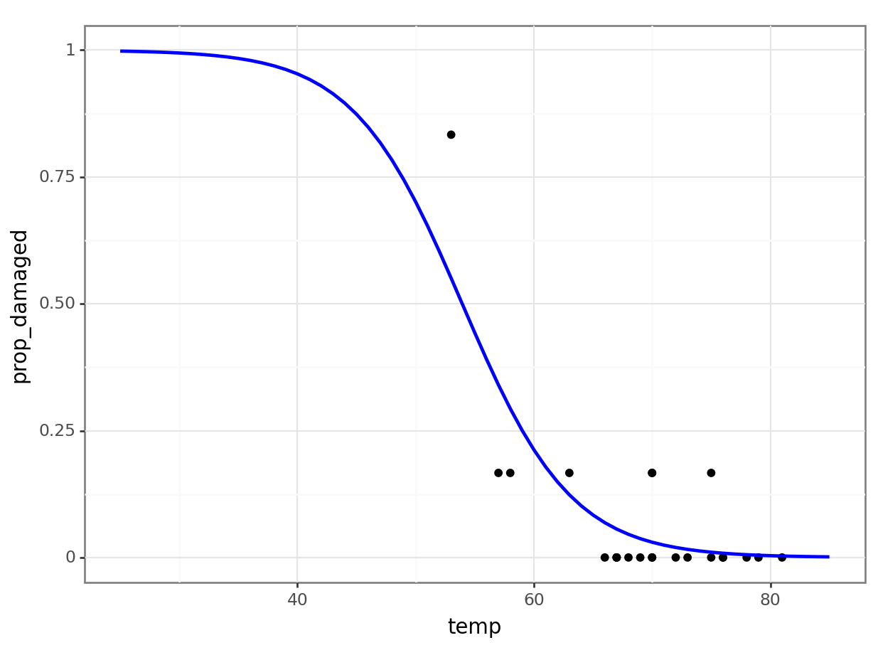
4 29 0.995469And let’s visualise the model:
(
  ggplot() +
     geom_point(challenger_py, aes(x = "temp", y = "prop_damaged")) +
     geom_line(model, aes(x = "temp", y = "pred"), colour = "blue", size = 1)
)
Comparing against the null
The next question we can ask is: is our model any better than the null model?
First we need to define the null model:
# create a linear model
model = smf.glm(formula = "damage + intact ~ 1",
                family = sm.families.Binomial(),
                data = challenger_py)
# and get the fitted parameters of the model
glm_chl_null_py = model.fit()

print(glm_chl_null_py.summary())
Generalized Linear Model Regression Results
================================================================================
Dep. Variable: ['damage', 'intact'] No. Observations: 23
Model: GLM Df Residuals: 22
Model Family: Binomial Df Model: 0
Link Function: Logit Scale: 1.0000
Method: IRLS Log-Likelihood: -25.830
Date: Wed, 09 Jul 2025 Deviance: 38.898
Time: 16:43:33 Pearson chi2: 58.5
No. Iterations: 5 Pseudo R-squ. (CS): 3.331e-16
Covariance Type: nonrobust
==============================================================================
coef std err z P>|z| [0.025 0.975]
------------------------------------------------------------------------------
Intercept -2.4463 0.314 -7.783 0.000 -3.062 -1.830
==============================================================================lrstat = -2*(glm_chl_null_py.llf - glm_chl_py.llf)
pvalue = chi2.sf(lrstat, glm_chl_null_py.df_resid - glm_chl_py.df_resid)
print(lrstat, pvalue)21.985381067707713 2.747351270353045e-06With a very small p-value (and a large chi-square statistic), it would seem that the model is indeed significantly better than the null.
Since there’s only one predictor variable, this is pretty much equivalent to saying that temp does predict the proportion of o-rings that are damaged.
So, could NASA have predicted what happened?
Probably, yes. They certainly should have listened to the engineers who were raising concerns based on these data. But that’s the subject of many documentaries, if you’re interested in the topic, so we won’t get into it here…
9.6.2 Predicting failure (with a tweak)
Exercise
Level:
In the challenger dataset, the data point at 53 degrees Fahrenheit is quite influential.
Would the conclusions from the previous exercise still hold without that point?
You should:
- Fit a model without this data point
- Visualise the new model
- Determine whether there is a significant link between launch temperature and o-ring failure in the new model
Answer
First, we need to remove the influential data point:
challenger_new <- challenger %>% filter(temp != 53)Now we can create a new generalised linear model, based on these data:
glm_chl_new <- glm(cbind(damage, intact) ~ temp,
               family = binomial,
               data = challenger_new)
We can get the model parameters as follows:
summary(glm_chl_new)
Call:
glm(formula = cbind(damage, intact) ~ temp, family = binomial,
data = challenger_new)
Coefficients:
Estimate Std. Error z value Pr(>|z|)
(Intercept) 5.68223 4.43138 1.282 0.1997
temp -0.12817 0.06697 -1.914 0.0556 .
---
Signif. codes: 0 '***' 0.001 '**' 0.01 '*' 0.05 '.' 0.1 ' ' 1
(Dispersion parameter for binomial family taken to be 1)
Null deviance: 16.375 on 21 degrees of freedom
Residual deviance: 12.633 on 20 degrees of freedom
AIC: 27.572
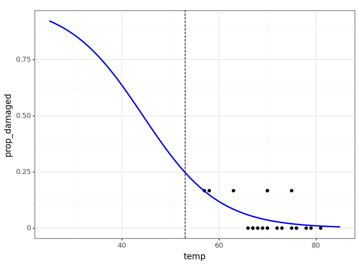
Number of Fisher Scoring iterations: 5And let’s visualise the model:
ggplot(challenger_new, aes(temp, prop_damaged)) +
  geom_point() +
  geom_smooth(method = "glm", se = FALSE, fullrange = TRUE,
              method.args = list(family = binomial)) +
  xlim(25,85) +
  # add a vertical line at 53 F temperature
  geom_vline(xintercept = 53, linetype = "dashed")
Warning in eval(family$initialize): non-integer #successes in a binomial glm!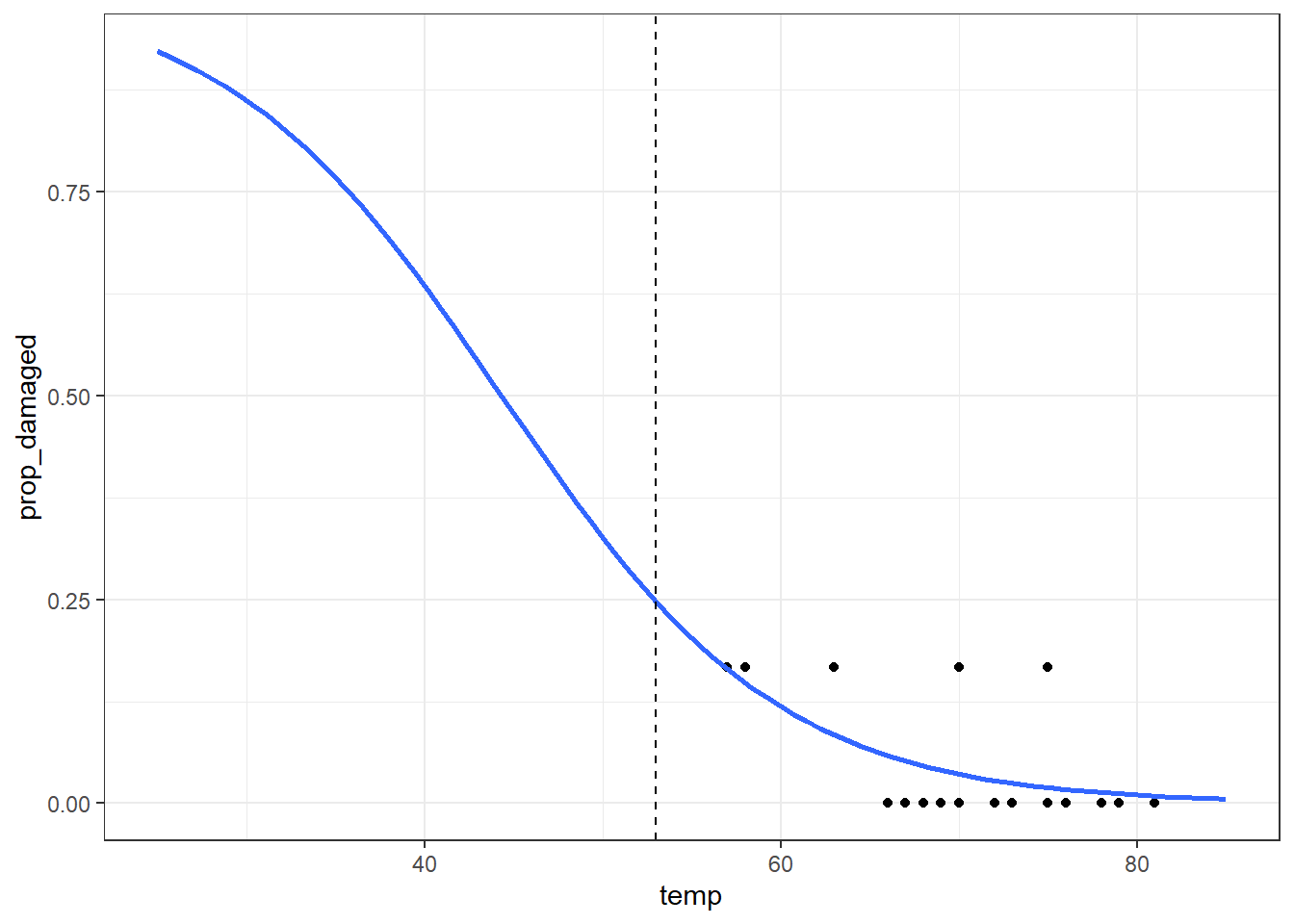
The prediction proportion of damaged o-rings is markedly less than what was observed.
Comparing against the null
So is our new model any better than the null?
We need to construct a new null model - we can’t use the one from the previous exercise, because it was fitted to a different dataset that had an extra observation.
glm_chl_null_new <- glm(cbind(damage, intact) ~ 1,
                family = binomial,
                data = challenger_new)

lrtest(glm_chl_new, glm_chl_null_new)
Likelihood ratio test
Model 1: cbind(damage, intact) ~ temp
Model 2: cbind(damage, intact) ~ 1
#Df LogLik Df Chisq Pr(>Chisq)
1 2 -11.786
2 1 -13.657 -1 3.7421 0.05306 .
---
Signif. codes: 0 '***' 0.001 '**' 0.01 '*' 0.05 '.' 0.1 ' ' 1The model is not significantly better than the null in this case, with a p-value here of just over 0.05.
First, we need to remove the influential data point:
challenger_new_py = challenger_py.query("temp != 53")We can create a new generalised linear model, based on these data:
# create a generalised linear model
model = smf.glm(formula = "damage + intact ~ temp",
                family = sm.families.Binomial(),
                data = challenger_new_py)
# and get the fitted parameters of the model
glm_chl_new_py = model.fit()
We can get the model parameters as follows:
print(glm_chl_new_py.summary()) Generalized Linear Model Regression Results
================================================================================
Dep. Variable: ['damage', 'intact'] No. Observations: 22
Model: GLM Df Residuals: 20
Model Family: Binomial Df Model: 1
Link Function: Logit Scale: 1.0000
Method: IRLS Log-Likelihood: -11.786
Date: Wed, 09 Jul 2025 Deviance: 12.633
Time: 16:43:34 Pearson chi2: 16.6
No. Iterations: 6 Pseudo R-squ. (CS): 0.1564
Covariance Type: nonrobust
==============================================================================
coef std err z P>|z| [0.025 0.975]
------------------------------------------------------------------------------
Intercept 5.6822 4.431 1.282 0.200 -3.003 14.368
temp -0.1282 0.067 -1.914 0.056 -0.259 0.003
==============================================================================Generate new model data:
model = pd.DataFrame({'temp': list(range(25, 86))})

model["pred"] = glm_chl_new_py.predict(model)

model.head()
temp pred
0 25 0.922585
1 26 0.912920
2 27 0.902177
3 28 0.890269
4 29 0.877107And let’s visualise the model:
(
  ggplot() +
     geom_point(challenger_new_py, aes(x = "temp", y = "prop_damaged")) +
     geom_line(model, aes(x = "temp", y = "pred"), colour = "blue", size = 1) +
     # add a vertical line at 53 F temperature
     geom_vline(xintercept = 53, linetype = "dashed")
)
The prediction proportion of damaged o-rings is markedly less than what was observed.
Comparing against the null
So is our new model any better than the null?
We need to construct a new null model - we can’t use the one from the previous exercise, because it was fitted to a different dataset that had an extra observation.
# create a linear model
model = smf.glm(formula = "damage + intact ~ 1",
                family = sm.families.Binomial(),
                data = challenger_new_py)
# and get the fitted parameters of the model
glm_chl_new_null_py = model.fit()

print(glm_chl_new_null_py.summary())
Generalized Linear Model Regression Results
================================================================================
Dep. Variable: ['damage', 'intact'] No. Observations: 22
Model: GLM Df Residuals: 21
Model Family: Binomial Df Model: 0
Link Function: Logit Scale: 1.0000
Method: IRLS Log-Likelihood: -13.657
Date: Wed, 09 Jul 2025 Deviance: 16.375
Time: 16:43:35 Pearson chi2: 16.8
No. Iterations: 6 Pseudo R-squ. (CS): -2.220e-16
Covariance Type: nonrobust
==============================================================================
coef std err z P>|z| [0.025 0.975]
------------------------------------------------------------------------------
Intercept -3.0445 0.418 -7.286 0.000 -3.864 -2.226
==============================================================================lrstat = -2*(glm_chl_new_null_py.llf - glm_chl_new_py.llf)
pvalue = chi2.sf(lrstat, glm_chl_new_null_py.df_resid - glm_chl_new_py.df_resid)
print(lrstat, pvalue)3.74211619353429 0.0530572082740162The model is not significantly better than the null in this case, with a p-value here of just over 0.05.
So, could NASA have predicted what happened? This model is not significantly different from the null, i.e., temperature is not a significant predictor.
However, note that it’s only marginally non-significant, and this is with a data point removed.
It is possible that if more data points were available that followed a similar trend, the story might be different). Even if we did use our non-significant model to make a prediction, it doesn’t give us a value anywhere near 5 failures for a temperature of 53 degrees Fahrenheit. So overall, based on the model we’ve fitted with these data, there was no clear indication that a temperature just a few degrees cooler than previous missions could have been so disastrous for the Challenger.
9.6.3 Revisiting rats and levers
Exercise
Level:
Last chapter, we fitted a model to the levers.csv dataset in Exercise 8.6.1.
Now, let’s test significance.
In this exercise, you should:
- Fit a model with the predictors
~ stress_type * sex + rat_age - Assess whether this model is significant over the null model
- Assess whether any of the 4 individual predictors (including the interaction) are significant
Answer
Fit the model
Before we fit the model, we need to:
- Read the data in
- Mutate to create an
incorrect_pressesvariable
levers <- read_csv("data/levers.csv")Rows: 62 Columns: 7
── Column specification ────────────────────────────────────────────────────────
Delimiter: ","
chr (2): stress_type, sex
dbl (5): rat_id, rat_age, trials, correct_presses, prop_correct
ℹ Use `spec()` to retrieve the full column specification for this data.
ℹ Specify the column types or set `show_col_types = FALSE` to quiet this message.levers <- levers %>%
mutate(incorrect_presses = trials - correct_presses)
glm_lev <- glm(cbind(correct_presses, incorrect_presses) ~ stress_type * sex + rat_age,
family = binomial,
data = levers)levers = pd.read_csv("data/levers.csv")
levers['incorrect_presses'] = levers['trials'] - levers['correct_presses']
model = smf.glm(formula = "correct_presses + incorrect_presses ~ stress_type * sex + rat_age",
family = sm.families.Binomial(),
data = levers)
glm_lev = model.fit()Compare to the null
We also need to fit a null model to these data before we can do any comparisons.
glm_lev_null <- glm(cbind(correct_presses, incorrect_presses) ~ 1,
                    family = binomial,
                    data = levers)
model = smf.glm(formula = "correct_presses + incorrect_presses ~ 1",
family = sm.families.Binomial(),
data = levers)
glm_lev_null = model.fit()Now, we run our likelihood ratio test comparing the two models.
anova(glm_lev, glm_lev_null)Analysis of Deviance Table
Model 1: cbind(correct_presses, incorrect_presses) ~ stress_type * sex +
rat_age
Model 2: cbind(correct_presses, incorrect_presses) ~ 1
Resid. Df Resid. Dev Df Deviance Pr(>Chi)
1 57 60.331
2 61 120.646 -4 -60.315 2.49e-12 ***
---
Signif. codes: 0 '***' 0.001 '**' 0.01 '*' 0.05 '.' 0.1 ' ' 1lrstat = -2*(glm_lev_null.llf - glm_lev.llf)
pvalue = chi2.sf(lrstat, glm_lev_null.df_resid - glm_lev.df_resid)
print(lrstat, pvalue)60.315193564424135 2.4904973429468967e-12This is pretty significant, suggesting that our model is quite a bit better than the null.
Test individual predictors
Now, let’s test individual predictors.
This is extremely easy to do in R. We produce an analysis of deviance table with anova, using the chi-square statistic for our likelihood ratios.
anova(glm_lev, test = "Chisq")Analysis of Deviance Table
Model: binomial, link: logit
Response: cbind(correct_presses, incorrect_presses)
Terms added sequentially (first to last)
Df Deviance Resid. Df Resid. Dev Pr(>Chi)
NULL 61 120.646
stress_type 1 8.681 60 111.965 0.0032150 **
sex 1 5.389 59 106.576 0.0202584 *
rat_age 1 12.216 58 94.359 0.0004738 ***
stress_type:sex 1 34.028 57 60.331 5.432e-09 ***
---
Signif. codes: 0 '***' 0.001 '**' 0.01 '*' 0.05 '.' 0.1 ' ' 1Let’s build two new candidate models: one with rat_age removed, and one with the stress:sex interaction removed.
(If the interaction isn’t significant, then we’ll push on and look at the main effects of stress and sex, if needed.)
The age effect
model = smf.glm(formula = "correct_presses + incorrect_presses ~ stress_type * sex",
                family = sm.families.Binomial(),
                data = levers)
glm_lev_dropage = model.fit()

lrstat = -2*(glm_lev_dropage.llf - glm_lev.llf)
pvalue = chi2.sf(lrstat, glm_lev_dropage.df_resid - glm_lev.df_resid)

print(lrstat, pvalue)
17.870581202609515 2.3644812834640866e-05The stress:sex interaction
model = smf.glm(formula = "correct_presses + incorrect_presses ~ stress_type + sex + rat_age",
                family = sm.families.Binomial(),
                data = levers)
glm_lev_dropint = model.fit()

lrstat = -2*(glm_lev_dropint.llf - glm_lev.llf)
pvalue = chi2.sf(lrstat, glm_lev_dropint.df_resid - glm_lev.df_resid)

print(lrstat, pvalue)
34.02832899366189 5.4315485567028665e-09Since the interaction is significant, we don’t really need the specifics of the main effects (it becomes hard to interpret!)
9.7 Summary
Likelihood and deviance are very important in generalised linear models - not just for fitting the model via maximum likelihood estimation, but for assessing significance and goodness-of-fit. To determine the quality of a model and draw conclusions from it, it’s important to assess both of these things.
Key points
- Deviance is the difference between predicted and actual values, and is calculated by comparing a model’s log-likelihood to that of the perfect “saturated” model
- Using deviance, likelihood ratio tests can be used in lieu of F-tests for generalised linear models
- This is distinct from (and often better than) using the Wald p-values that are reported automatically in the model summary