install.packages("lmtest")
library(lmtest)10 Goodness-of-fit
Goodness-of-fit is all about how well a model fits the data, and typically involves summarising the discrepancy between the actual data points, and the fitted/predicted values that the model produces.
Though closely linked, it’s important to realise that goodness-of-fit and significance don’t come hand-in-hand automatically: we might find a model that is significantly better than the null, but is still overall pretty rubbish at matching the data. So, to understand the quality of our model better, we should ideally perform both types of test.
Learning outcomes
- Understand the difference between significance and goodness-of-fit
- Know how to use at least two methods to evaluate the quality of a model fit
- Know how to use AIC values to perform model comparison
10.1 Libraries and functions
Click to expand
from scipy.stats import *10.2 Data and model
We’ll continue using the data and model for the diabetes dataset, which were defined as follows:
diabetes <- read_csv("data/diabetes.csv")Rows: 728 Columns: 3
── Column specification ────────────────────────────────────────────────────────
Delimiter: ","
dbl (3): glucose, diastolic, test_result
ℹ Use `spec()` to retrieve the full column specification for this data.
ℹ Specify the column types or set `show_col_types = FALSE` to quiet this message.glm_dia <- glm(test_result ~ glucose * diastolic,
family = "binomial",
data = diabetes)
glm_null <- glm(test_result ~ 1,
family = binomial,
data = diabetes)diabetes_py = pd.read_csv("data/diabetes.csv")model = smf.glm(formula = "test_result ~ glucose * diastolic",
family = sm.families.Binomial(),
data = diabetes_py)
glm_dia_py = model.fit()
model = smf.glm(formula = "test_result ~ 1",
family = sm.families.Binomial(),
data = diabetes_py)
glm_null_py = model.fit()10.3 Chi-square tests
Last chapter, we talked about deviance and chi-square tests, to assess significance.
We can use these in a very similar way to assess the goodness-of-fit of a model.
When we compared our model against the null (last chapter), we tested the null hypothesis that the candidate model and the null model had the same deviance.
Now, however, we will test the null hypothesis that the fitted model and the saturated (perfect) model have the same deviance, i.e., that they both fit the data equally well.
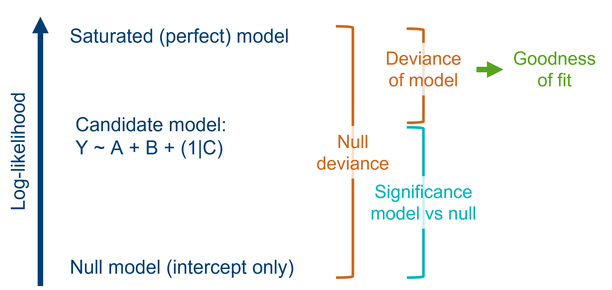
In most hypothesis tests, we want to reject the null hypothesis, but in this case, we’d like it to be true.
Running a goodness-of-fit chi-square test in R can be done using the pchisq function. We need to include two arguments: 1) the residual deviance, and 2) the residual degrees of freedom. Both of these can be found in the summary output, but you can use the $ syntax to call these properties directly like so:
pchisq(glm_dia$deviance, glm_dia$df.residual, lower.tail = FALSE)[1] 0.2605931The syntax is very similar to the LRT we ran above, but now instead of including information about both our candidate model and the null, we instead just need 1) the residual deviance, and 2) the residual degrees of freedom:
pvalue = chi2.sf(glm_dia_py.deviance, glm_dia_py.df_resid)

print(pvalue)0.26059314630406843You can think about this p-value, roughly, as “the probability that this model is good”. We’re not below our significance threshold, which means that we’re not rejecting our null hypothesis (which is a good thing) - but it’s also not a huge probability. This suggests that there’s probably other variables we could measure and include in a future experiment, to give a better overall model.
10.4 AIC values
You might remember AIC values from standard linear modelling. AIC values are useful, because they tell us about overall model quality, factoring in both goodness-of-fit and model complexity.
One of the best things about the Akaike information criterion (AIC) is that it isn’t specific to linear models - it works for models fitted with maximum likelihood estimation.
In fact, if you look at the formula for AIC, you’ll see why:
\[ AIC = 2k - 2ln(\hat{L}) \]
where \(k\) represents the number of parameters in the model, and \(\hat{L}\) is the maximised likelihood function. In other words, the two parts of the equation represent the complexity of the model, versus the log-likelihood.
This means that AIC can be used for model comparison for GLMs in precisely the same way as it’s used for linear models: lower AIC indicates a better-quality model.
The AIC value is given as standard, near the bottom of the summary output (just below the deviance values). You can also print it directly using the $ syntax:
summary(glm_dia)
Call:
glm(formula = test_result ~ glucose * diastolic, family = "binomial",
    data = diabetes)

Coefficients:
                    Estimate Std. Error z value Pr(>|z|)
(Intercept)       -8.5710565  2.7032318  -3.171  0.00152 **
glucose            0.0547050  0.0209256   2.614  0.00894 **
diastolic          0.0423651  0.0363681   1.165  0.24406
glucose:diastolic -0.0002221  0.0002790  -0.796  0.42590
---
Signif. codes:  0 '***' 0.001 '**' 0.01 '*' 0.05 '.' 0.1 ' ' 1

(Dispersion parameter for binomial family taken to be 1)

    Null deviance: 936.60  on 727  degrees of freedom
Residual deviance: 748.01  on 724  degrees of freedom
AIC: 756.01

Number of Fisher Scoring iterations: 4glm_dia$aic[1] 756.0069In even better news for R users, the step function works for GLMs just as it does for linear models, so long as you include the test = LRT argument.
step(glm_dia, test = "LRT")Start: AIC=756.01
test_result ~ glucose * diastolic
Df Deviance AIC LRT Pr(>Chi)
- glucose:diastolic 1 748.64 754.64 0.62882 0.4278
<none> 748.01 756.01
Step: AIC=754.64
test_result ~ glucose + diastolic
Df Deviance AIC LRT Pr(>Chi)
<none> 748.64 754.64
- diastolic 1 752.20 756.20 3.564 0.05905 .
- glucose 1 915.52 919.52 166.884 < 2e-16 ***
---
Signif. codes: 0 '***' 0.001 '**' 0.01 '*' 0.05 '.' 0.1 ' ' 1
Call:  glm(formula = test_result ~ glucose + diastolic, family = "binomial",
    data = diabetes)

Coefficients:
(Intercept)      glucose    diastolic
   -6.49941      0.03836      0.01407

Degrees of Freedom: 727 Total (i.e. Null);  725 Residual
Null Deviance:      936.6
Residual Deviance: 748.6    AIC: 754.6
The AIC value isn’t printed as standard with the model summary, but you can access it easily like so:
print(glm_dia_py.aic)756.006858606974410.5 Pseudo \(R^2\)
Refresher on \(R^2\)
In linear modelling, we could extract and interpret \(R^2\) values that summarised our model. \(R^2\) in linear modelling represents a few different things:
- The proportion of variance in the response variable, that’s explained by the model (i.e., jointly by the predictors)
- The improvement of the model over the null model
- The square of the Pearson’s correlation coefficient
The first one on that list is the interpretation we usually use it for, in linear modelling.
What is a “pseudo \(R^2\)”?
It’s not possible to calculate \(R^2\) for a GLM like you can for a linear model.
However, because people are fond of using \(R^2\), statisticians have developed alternatives that can be used instead.
There is no single value that can replace \(R^2\) and have all the same interpretations, so several different metrics have been proposed. Depending how they’re calculated, they all have different interpretations.
There are many. Some of the most popular are McFadden’s, Nagelkerke’s, Cox & Snell’s, and Tjur’s. This post does a nice job of discussing some of them and providing some comparisons.
Should you use pseudo \(R^2\)?
We recommend not to use pseudo \(R^2\).
(Unless you are very statistically-minded and prepared to wade through a lot of mathematical explanation…)
This is for a few reasons:
- It’s too easy to fall into the bad habit of treating it like regular \(R^2\), and making bad interpretations
- Even if you’ve done a good job, your readers might make their own bad interpretations
- Figuring out which version to use, and what they all mean, is a minefield
- It doesn’t really tell you anything that a chi-square test and/or AIC can’t tell you
The main reason we’ve mentioned it here is because you are likely to come across pseudo \(R^2\) when reading research papers that use GLMs - we want you to know what they are!
10.6 Exercises
10.6.1 Revisiting aphids
Exercise
Level:
Back in Exercise 7.7.2, we fitted a logistic model to the aphids dataset - the code is included below in case you need to run it again.
Now, let’s assess the goodness-of-fit of that model.
You should:
- Compute a chi-square goodness-of-fit test for the full model (
~ buds + cultivar) - Calculate the AIC value for the full model
- Use backwards stepwise elimination to determine whether dropping the
budsand/orcultivarpredictors improves the goodness-of-fit
aphids <- read_csv("data/aphids.csv")

glm_aphids <- glm(aphids_present ~ buds + cultivar,
                  family = binomial,
                  data = aphids)
aphids = pd.read_csv("data/aphids.csv")
model = smf.glm(formula = "aphids_present ~ buds + cultivar",
family = sm.families.Binomial(),
data = aphids)
glm_aphids = model.fit()
Answer
Chi-square goodness-of-fit
This is a simple one-function task:
pchisq(glm_aphids$deviance, glm_aphids$df.residual, lower.tail = FALSE)[1] 0.1666178The syntax is very similar to the LRT we ran above, but now instead of including information about both our candidate model and the null, we instead just need 1) the residual deviance, and 2) the residual degrees of freedom:
pvalue = chi2.sf(glm_aphids.deviance, glm_aphids.df_resid)

print(pvalue)0.16661777677427902Extract AIC for full model
We can access the AIC either in the model summary:
summary(glm_aphids)
Call:
glm(formula = aphids_present ~ buds + cultivar, family = binomial,
    data = aphids)

Coefficients:
               Estimate Std. Error z value Pr(>|z|)
(Intercept)     -2.0687     0.7483  -2.765  0.00570 **
buds             0.2067     0.1262   1.638  0.10149
cultivarmozart   1.9621     0.6439   3.047  0.00231 **
---
Signif. codes:  0 '***' 0.001 '**' 0.01 '*' 0.05 '.' 0.1 ' ' 1

(Dispersion parameter for binomial family taken to be 1)

    Null deviance: 73.670  on 53  degrees of freedom
Residual deviance: 60.666  on 51  degrees of freedom
AIC: 66.666

Number of Fisher Scoring iterations: 4
or directly using the $ syntax:
glm_aphids$aic[1] 66.66602The AIC value is an “attribute” of the model object, which we can access like so:
print(glm_aphids.aic)66.66602340347231Backwards stepwise elimination
Last but not least, let’s see if dropping either or both of the predictors improves the model quality. (Spoiler: it probably won’t!)
We use the convenient step function for this - don’t forget the test = LRT argument, though.
step(glm_dia, test = "LRT")Start: AIC=756.01
test_result ~ glucose * diastolic
Df Deviance AIC LRT Pr(>Chi)
- glucose:diastolic 1 748.64 754.64 0.62882 0.4278
<none> 748.01 756.01
Step: AIC=754.64
test_result ~ glucose + diastolic
Df Deviance AIC LRT Pr(>Chi)
<none> 748.64 754.64
- diastolic 1 752.20 756.20 3.564 0.05905 .
- glucose 1 915.52 919.52 166.884 < 2e-16 ***
---
Signif. codes: 0 '***' 0.001 '**' 0.01 '*' 0.05 '.' 0.1 ' ' 1
Call:  glm(formula = test_result ~ glucose + diastolic, family = "binomial",
    data = diabetes)

Coefficients:
(Intercept)      glucose    diastolic
   -6.49941      0.03836      0.01407

Degrees of Freedom: 727 Total (i.e. Null);  725 Residual
Null Deviance:      936.6
Residual Deviance: 748.6    AIC: 754.6
Since neither of our reduced models improve on the AIC versus our original model, we don’t drop either predictor, and the process stops there.
We need to build two new candidate models. In each case, we drop just one variable.
# Dropping buds
model = smf.glm(formula = "aphids_present ~ cultivar",
                family = sm.families.Binomial(),
                data = aphids)

glm_aphids_dropbuds = model.fit()

# Dropping cultivar
model = smf.glm(formula = "aphids_present ~ buds",
                family = sm.families.Binomial(),
                data = aphids)

glm_aphids_dropcultivar = model.fit()
Now, we can look at the three AIC values next to each other, to determine which of these is the best option.
print(glm_aphids.aic,
      glm_aphids_dropbuds.aic,
      glm_aphids_dropcultivar.aic)
66.66602340347231 67.51106908352895 75.19195097185758Since neither of our reduced models improve on the AIC versus our original model, we don’t drop either predictor, and the process stops there.
10.7 Summary
Likelihood and deviance are very important in generalised linear models - not just for fitting the model via maximum likelihood estimation, but for assessing significance and goodness-of-fit. To determine the quality of a model and draw conclusions from it, it’s important to assess both of these things.
Key points
- A chi-square goodness-of-fit test can also be performed using likelihood/deviance
- The Akaike information criterion is also based on likelihood, and can be used to compare the quality of GLMs fitted to the same dataset
- Other metrics that may be of use are Wald test p-values and pseudo \(R^2\) values (if interpreted thoughtfully)