13 Overdispersed count data

Learning outcomes

Understand what dispersion is and why it’s important
Be able to diagnose or recognise overdispersion in count data
Fit a negative binomial regression model to overdispersed count data
Know the difference between Poisson and negative binomial regression
Assess whether assumptions are met and evaluate fit of a negative binomial model

13.1 Libraries and functions

Click to expand

R
Python

13.1.1 Libraries

library(MASS)
library(performance)
library(tidyverse)
library(broom)

13.1.2 Libraries

# A maths library
import math
import pandas as pd
from plotnine import *
import statsmodels.api as sm
import statsmodels.formula.api as smf
from scipy.stats import *
import numpy as np
from statsmodels.discrete.discrete_model import NegativeBinomial

13.2 Removing dispersion assumptions

In the previous chapter we looked at how to analyse count data. We used a Poisson regression to do this, which makes the assumption that the dispersion parameter \(\approx 1\) (for a refresher on dispersion, see Section 12.6).

So what happens if the data is over- or under-dispersed?

Cue negative binomial models.

Negative binomial models are also used for count data, but they have one crucial difference from Poisson regression: instead of making an assumption about the dispersion parameter, they actually estimate it as part of the model fitting.

13.3 Parasites dataset

We’ll explore this with the parasites dataset.

These data are about parasites found on the gills of freshwater fish.

The ecologists who conducted the research observed a total of 64 fish, which varied by:

which lake they were found in
the fish_length (cm)

They were interested in how these factors influenced the parasite_count of small parasites found on each fish.

13.4 Load and visualise the data

First we load the data, then we visualise it.

R
Python

parasites <- read_csv("data/parasites.csv")

head(parasites)

# A tibble: 6 × 3
  parasite_count lake  fish_length
           <dbl> <chr>       <dbl>
1             46 C            21.1
2            138 C            26.4
3             23 C            18.9
4             35 B            27.2
5            118 C            29  
6             43 B            24.2

ggplot(parasites, aes(y = parasite_count, x = fish_length, colour = lake)) +
  geom_point()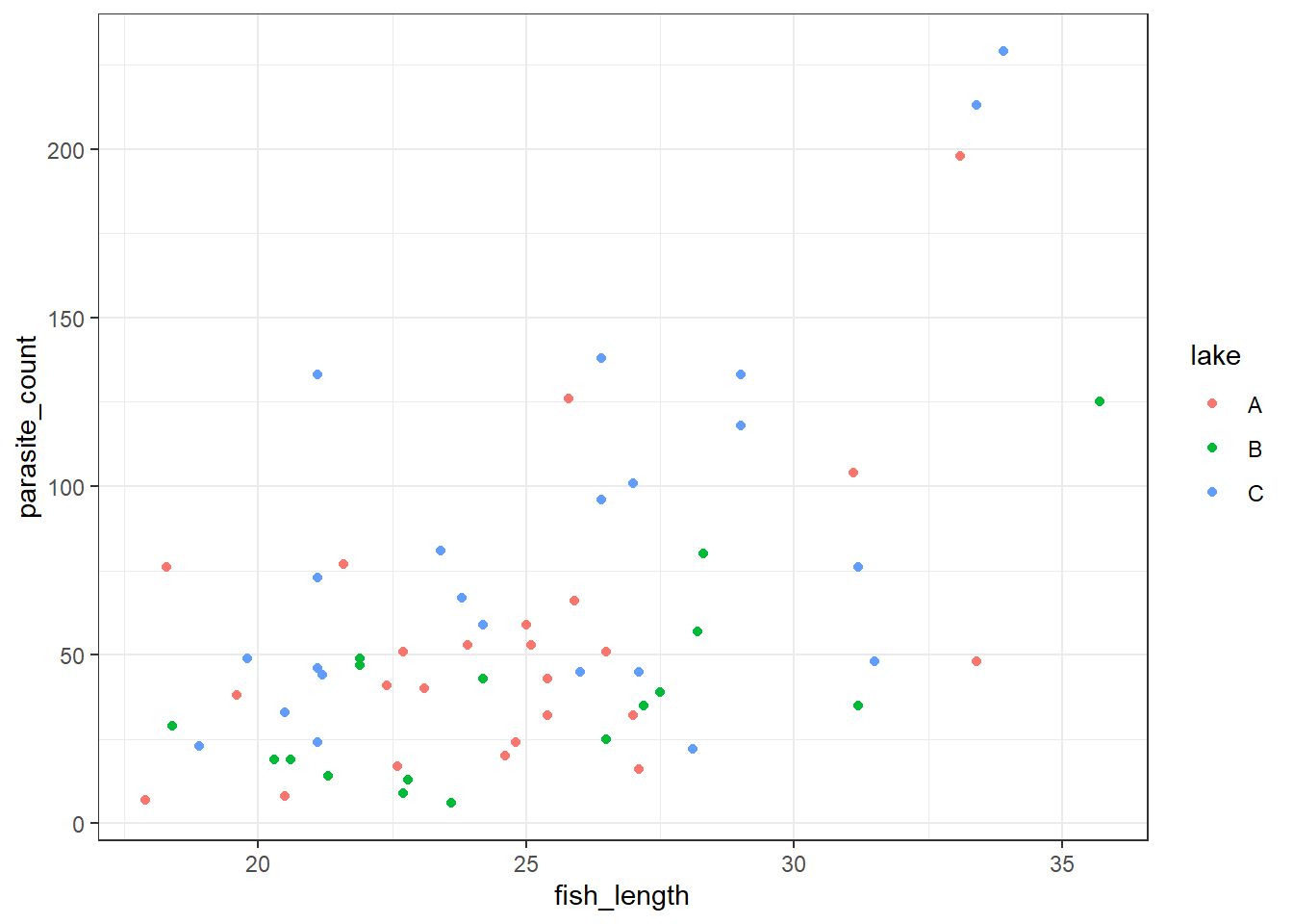

ggplot(parasites, aes(y = parasite_count, x = lake, colour = fish_length)) +
  geom_violin() +
  geom_jitter()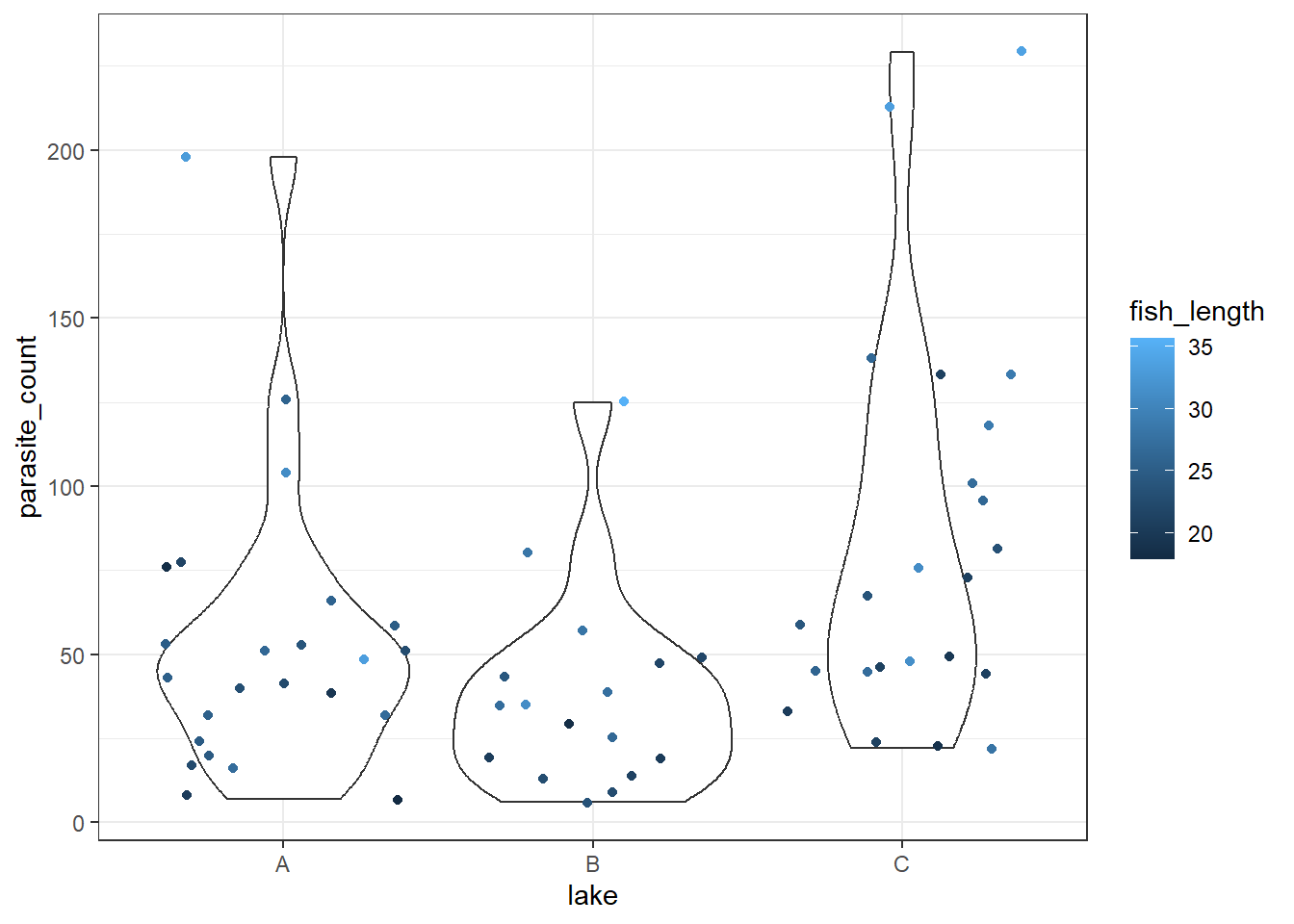

parasites = pd.read_csv("data/parasites.csv")

parasites.head()

   parasite_count lake  fish_length
0              46    C         21.1
1             138    C         26.4
2              23    C         18.9
3              35    B         27.2
4             118    C         29.0

(
  ggplot(parasites, aes(y = "parasite_count", x = "fish_length", colour = "lake")) +
  geom_point()
)

<Figure Size: (640 x 480)>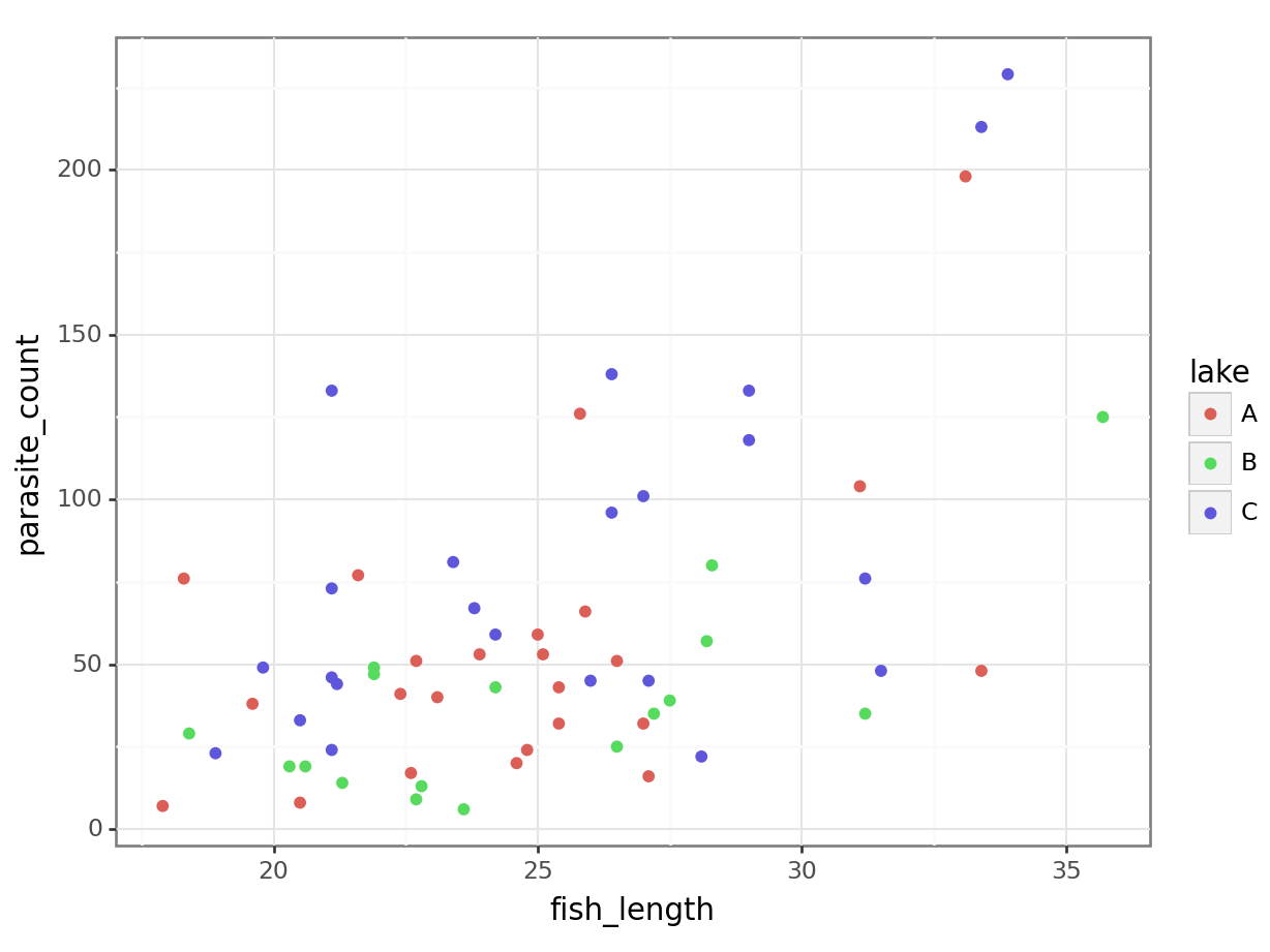

(
  ggplot(parasites, aes(y = "parasite_count", x = "lake", colour = "fish_length")) +
  geom_violin() +
  geom_jitter()
)

<Figure Size: (640 x 480)>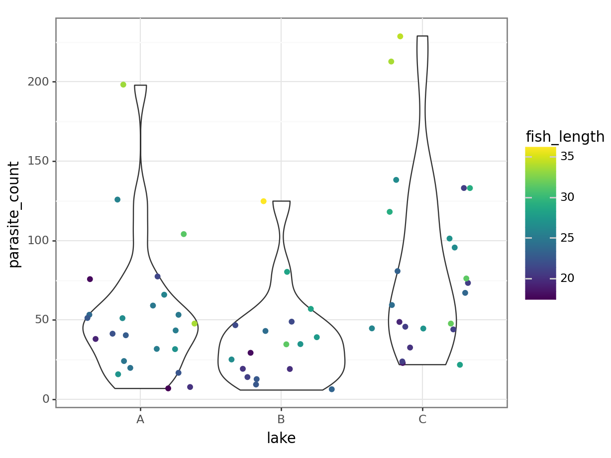

We get a reasonably clear picture here; it seems that lake C might have a higher number of parasites overall, and that across all three lakes, bigger fish have more parasites too.

13.5 Constructing a Poisson model

Given that the response variable, parasite_count, is a count variable, let’s try to construct a Poisson regression.

We’ll construct the full model, with an interaction.

R
Python

glm_para <- glm(parasite_count ~ lake * fish_length,
                data = parasites, family = "poisson")

and we look at the model summary:

summary(glm_para)


Call:
glm(formula = parasite_count ~ lake * fish_length, family = "poisson", 
    data = parasites)

Coefficients:
                    Estimate Std. Error z value Pr(>|z|)    
(Intercept)        1.656e+00  1.763e-01   9.391   <2e-16 ***
lakeB             -7.854e-01  2.804e-01  -2.801   0.0051 ** 
lakeC              3.527e-01  2.261e-01   1.560   0.1188    
fish_length        9.127e-02  6.643e-03  13.738   <2e-16 ***
lakeB:fish_length  1.523e-02  1.031e-02   1.477   0.1398    
lakeC:fish_length -5.079e-05  8.389e-03  -0.006   0.9952    
---
Signif. codes:  0 '***' 0.001 '**' 0.01 '*' 0.05 '.' 0.1 ' ' 1

(Dispersion parameter for poisson family taken to be 1)

    Null deviance: 2073.8  on 63  degrees of freedom
Residual deviance: 1056.5  on 58  degrees of freedom
AIC: 1429.2

Number of Fisher Scoring iterations: 5

model = smf.glm(formula = "parasite_count ~ lake * fish_length",
                family = sm.families.Poisson(),
                data = parasites)

glm_para = model.fit()

Let’s look at the model output:

print(glm_para.summary())

                 Generalized Linear Model Regression Results                  
==============================================================================
Dep. Variable:         parasite_count   No. Observations:                   64
Model:                            GLM   Df Residuals:                       58
Model Family:                 Poisson   Df Model:                            5
Link Function:                    Log   Scale:                          1.0000
Method:                          IRLS   Log-Likelihood:                -708.61
Date:                Thu, 10 Jul 2025   Deviance:                       1056.5
Time:                        13:49:02   Pearson chi2:                 1.07e+03
No. Iterations:                     5   Pseudo R-squ. (CS):              1.000
Covariance Type:            nonrobust                                         
=========================================================================================
                            coef    std err          z      P>|z|      [0.025      0.975]
-----------------------------------------------------------------------------------------
Intercept                 1.6556      0.176      9.391      0.000       1.310       2.001
lake[T.B]                -0.7854      0.280     -2.801      0.005      -1.335      -0.236
lake[T.C]                 0.3527      0.226      1.560      0.119      -0.090       0.796
fish_length               0.0913      0.007     13.738      0.000       0.078       0.104
lake[T.B]:fish_length     0.0152      0.010      1.477      0.140      -0.005       0.035
lake[T.C]:fish_length -5.079e-05      0.008     -0.006      0.995      -0.016       0.016
=========================================================================================

13.5.1 Checking dispersion

Before we launch into any significance testing, we’re going to check one of the assumptions: that the dispersion parameter = 1 (you might’ve guessed where this is going…)

R
Python

check_overdispersion(glm_para)

# Overdispersion test

       dispersion ratio =   18.378
  Pearson's Chi-Squared = 1065.905
                p-value =  < 0.001

Overdispersion detected.

print(glm_para.deviance/glm_para.df_resid)

18.215417572845304

pvalue = chi2.sf(glm_para.deviance, glm_para.df_resid)
print(pvalue)

2.312587481511686e-183

Oh no - there is definitely overdispersion here.

We won’t bother looking at the analysis of deviance table or asking whether the model is better than the null model. The Poisson regression we’ve fitted here is not right, and we need to fit a different type of model.

The main alternative to a Poisson model, used for overdispersed count data, is something called a negative binomial model.

To specify a negative binomial model, we use the glm.nb function from the MASS package.

The syntax is the same as glm, except we don’t need to specify a family argument.

nb_para <- glm.nb(parasite_count ~ lake * fish_length, parasites)

summary(nb_para)


Call:
glm.nb(formula = parasite_count ~ lake * fish_length, data = parasites, 
    init.theta = 3.37859216, link = log)

Coefficients:
                   Estimate Std. Error z value Pr(>|z|)   
(Intercept)        1.943370   0.739434   2.628  0.00858 **
lakeB             -0.784885   1.094625  -0.717  0.47335   
lakeC              0.212060   1.006021   0.211  0.83305   
fish_length        0.079939   0.029485   2.711  0.00671 **
lakeB:fish_length  0.015428   0.043380   0.356  0.72210   
lakeC:fish_length  0.005719   0.039542   0.145  0.88501   
---
Signif. codes:  0 '***' 0.001 '**' 0.01 '*' 0.05 '.' 0.1 ' ' 1

(Dispersion parameter for Negative Binomial(3.3786) family taken to be 1)

    Null deviance: 118.202  on 63  degrees of freedom
Residual deviance:  67.288  on 58  degrees of freedom
AIC: 615.99

Number of Fisher Scoring iterations: 1

              Theta:  3.379 
          Std. Err.:  0.623 

 2 x log-likelihood:  -601.991

This output is very similar to the other GLM outputs that we’ve seen but with some additional information at the bottom regarding the dispersion parameter that the negative binomial model has used, which in R is called theta (\(\theta\)), 3.379.

This number is estimated from the data. This is what makes negative binomial regression different from Poisson regression.

We can continue to use statsmodels, specifically the NegativeBinomial function.

The syntax for getting this to work is a little different, and takes several steps.

First, we identify our response variable:

Y = parasites['parasite_count']

Now, we need to set up our set of predictors. The function we’re using requires us to provide a matrix where each row is a unique observation (fish, in this case) and each column is a predictor.

Because we want to include the lake:fish_length interaction, we actually need to manually generate those columns ourselves, like this:

# 1. Create dummy variables for 'lake' (switch to True/False values)
lake_dummies = pd.get_dummies(parasites['lake'], drop_first=True)

# 2. Create interaction terms manually: lake_dummies * fish_length
interactions = lake_dummies.multiply(parasites['fish_length'], axis=0)
interactions.columns = [f'{col}:fish_length' for col in interactions.columns]

# 3. Combine all predictors: fish_length, lake dummies, interactions
X = pd.concat([parasites['fish_length'], lake_dummies, interactions], axis=1)

# 4. Add a constant/intercept (required), and make sure that we're using floats
X = sm.add_constant(X).astype(float)

Now, we can fit our model and look at the summary:

from statsmodels.discrete.discrete_model import NegativeBinomial

# Specify the model (Y, X)
model = NegativeBinomial(Y, X)

nb_para = model.fit()

Optimization terminated successfully.
         Current function value: 4.703057
         Iterations: 32
         Function evaluations: 39
         Gradient evaluations: 39

print(nb_para.summary())

                     NegativeBinomial Regression Results                      
==============================================================================
Dep. Variable:         parasite_count   No. Observations:                   64
Model:               NegativeBinomial   Df Residuals:                       58
Method:                           MLE   Df Model:                            5
Date:                Thu, 10 Jul 2025   Pseudo R-squ.:                 0.05947
Time:                        13:49:03   Log-Likelihood:                -301.00
converged:                       True   LL-Null:                       -320.03
Covariance Type:            nonrobust   LLR p-value:                 3.658e-07
=================================================================================
                    coef    std err          z      P>|z|      [0.025      0.975]
---------------------------------------------------------------------------------
const             1.9434      0.689      2.819      0.005       0.592       3.294
fish_length       0.0799      0.027      2.915      0.004       0.026       0.134
B                -0.7849      1.026     -0.765      0.444      -2.796       1.226
C                 0.2121      0.961      0.221      0.825      -1.671       2.095
B:fish_length     0.0154      0.041      0.380      0.704      -0.064       0.095
C:fish_length     0.0057      0.038      0.152      0.879      -0.068       0.080
alpha             0.2960      0.055      5.424      0.000       0.189       0.403
=================================================================================

In particular, we might like to know what the dispersion parameter is.

By default, NegativeBinomial from statsmodels provides something called alpha (\(\alpha\)), which is not the same as the significance threshold. To convert this into the dispersion parameter you’re using to seeing (sometimes referred to as theta, \(\theta\)), you need \(\frac{1}{\alpha}\).

print(1/nb_para.params['alpha'])

3.3785919925485657

13.6.1 Extract equation

If we wanted to express our model as a formal equation, we need to extract the coefficients:

R
Python

coefficients(nb_para)

      (Intercept)             lakeB             lakeC       fish_length 
      1.943370195      -0.784885086       0.212060149       0.079939234 
lakeB:fish_length lakeC:fish_length 
      0.015428470       0.005718571

print(nb_para.params)

const            1.943370
fish_length      0.079939
B               -0.784885
C                0.212060
B:fish_length    0.015428
C:fish_length    0.005719
alpha            0.295981
dtype: float64

These are the coefficients of the negative binomial model equation and need to be placed in the following formula in order to estimate the expected number of species as a function of the other variables:

\[ \begin{split} E(species) = \exp(1.94 + \begin{pmatrix} 0 \\ -0.78 \\ 0.212 \end{pmatrix} \begin{pmatrix} A \\ B \\ C \end{pmatrix} + 0.08 \times fishlength + \begin{pmatrix} 0 \\ 0.0154 \\ 0.0057 \end{pmatrix} \begin{pmatrix} A \\ B \\ C \end{pmatrix} \times fishlength) \end{split} \]

13.6.2 Comparing Poisson and negative binomial

The main difference between a Poisson regression and a negative binomial regression is this: in the former the dispersion parameter is assumed to be 1, whereas in the latter it is estimated from the data.

They both, however, use the same link function - the log link function.

This means they will both have equations in the same form, as we just showed above. It also means that they can produce some quite similar-looking models.

Let’s visualise and compare them.

First, let’s plot the Poisson model:

R
Python

ggplot(parasites, aes(y = parasite_count, x = fish_length, colour = lake)) +
  geom_point() +
  geom_smooth(method = "glm", se = FALSE, fullrange = TRUE, 
              method.args = list(family = "poisson"))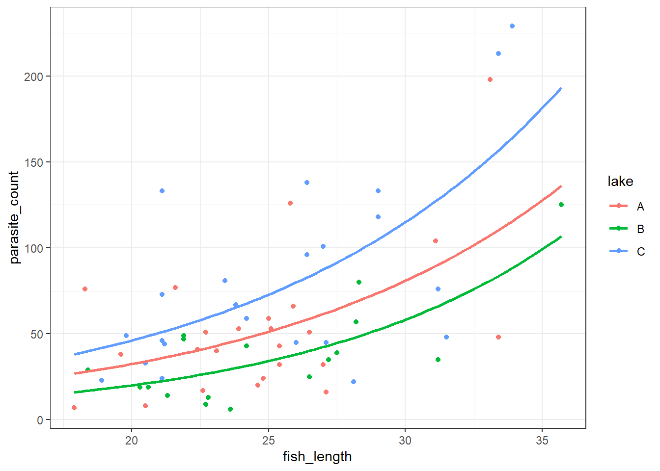

To do this, we need to produce a set of predictions, which we can then plot.

# Get unique lake values from your dataset
lake_levels = parasites['lake'].unique()

# Create prediction grid for each lake
new_data = pd.concat([
    pd.DataFrame({
        'fish_length': np.linspace(10, 40, 100),
        'lake': lake
    }) for lake in lake_levels
])

# Predict
new_data['pred'] = glm_para.predict(new_data)

new_data.head()

   fish_length lake       pred
0    10.000000    C  18.549643
1    10.303030    C  19.069529
2    10.606061    C  19.603986
3    10.909091    C  20.153422
4    11.212121    C  20.718257

(
  ggplot(parasites,
         aes(x = "fish_length",
             y = "parasite_count",
             colour = "lake")) +
     geom_point() +
     geom_line(new_data, aes(x = "fish_length", y = "pred", colour = "lake"), size = 1)
)

<Figure Size: (640 x 480)>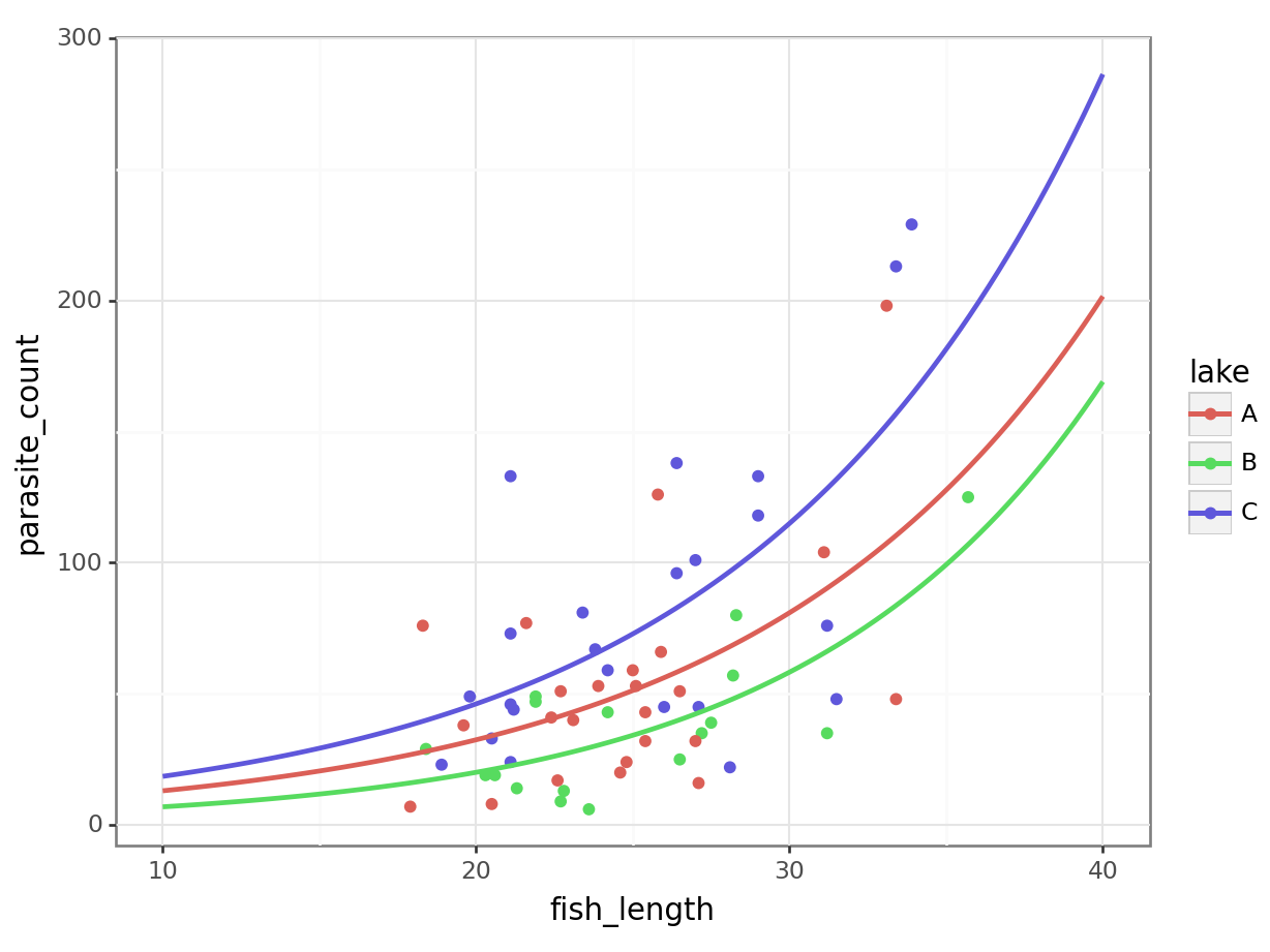

Now, let’s plot the negative binomial model:

R
Python

All we have to do is switch the method for geom_smooth over to glm.nb:

ggplot(parasites, aes(y = parasite_count, x = fish_length, colour = lake)) +
  geom_point() +
  geom_smooth(method = "glm.nb", se = FALSE, fullrange = TRUE)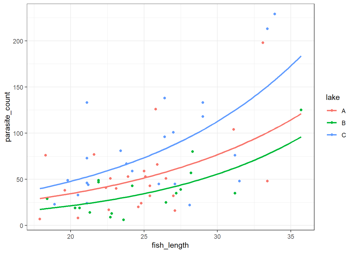

# Get unique lake values from your dataset
lake_levels = parasites['lake'].unique()

# Create prediction grid for each lake
new_data_nb = pd.concat([
    pd.DataFrame({
        'fish_length': np.linspace(10, 40, 100),
        'lake': lake
    }) for lake in lake_levels
])

# Repeat the transformations we used when fitting the model
lake_dummies = pd.get_dummies(new_data['lake'], drop_first=True)
interactions = lake_dummies.multiply(new_data_nb['fish_length'], axis=0)
interactions.columns = [f'{col}:fish_length' for col in interactions.columns]
X_new = pd.concat([new_data_nb['fish_length'], lake_dummies, interactions], axis=1)
X_new = sm.add_constant(X_new).astype(float)

# Now we can safely predict:
new_data_nb['pred'] = nb_para.predict(X_new)

new_data_nb.head()

   fish_length lake       pred
0    10.000000    C  20.328185
1    10.303030    C  20.862750
2    10.606061    C  21.411372
3    10.909091    C  21.974421
4    11.212121    C  22.552276

(
  ggplot(parasites,
         aes(x = "fish_length",
             y = "parasite_count",
             colour = "lake")) +
     geom_point() +
     geom_line(new_data_nb, aes(x = "fish_length", y = "pred", colour = "lake"), size = 1)
)

<Figure Size: (640 x 480)>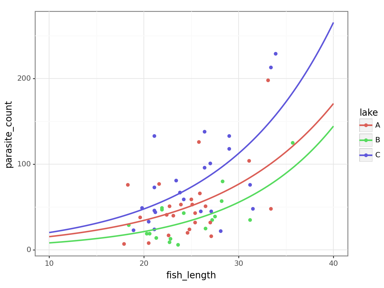

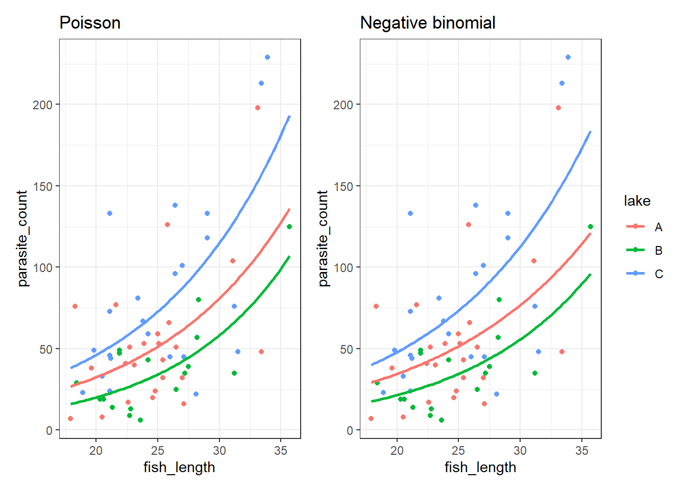
It’s subtle - the two sets of curves look quite similar - but they’re not quite the same.

Looking at them side-by-side may help:

13.6.3 Checking assumptions & model quality

These steps are performed in precisely the same way we would do for a Poisson regression.

Remember, the things we checked for in a Poisson regression were:

Response distribution
Correct link function
Independence
Influential points
Collinearity
Dispersion

For free, I’ll just tell you now that the first three assumptions are met.

Plus, we don’t have to worry about dispersion with a negative binomial model.

So, all we really need to pay attention to is whether there are any influential points to worry about, or any collinearity.

R
Python

Once again, the performance package comes in handy for assessing all of these.

check_model(nb_para, check = c('pp_check',
                               'vif',
                               'outliers'))

Cannot simulate residuals for models of class `negbin`. Please try
  `check_model(..., residual_type = "normal")` instead.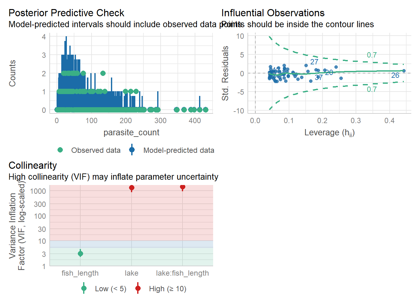

check_outliers(nb_para, threshold = list('cook'=0.5))

OK: No outliers detected.
- Based on the following method and threshold: cook (0.5).
- For variable: (Whole model)

check_collinearity(nb_para)

Model has interaction terms. VIFs might be inflated.
  Try to center the variables used for the interaction, or check
  multicollinearity among predictors of a model without interaction terms.

# Check for Multicollinearity

Low Correlation

        Term  VIF        VIF 95% CI Increased SE Tolerance Tolerance 95% CI
 fish_length 3.13 [  2.26,    4.61]         1.77      0.32     [0.22, 0.44]

High Correlation

             Term     VIF        VIF 95% CI Increased SE Tolerance
             lake 1321.85 [863.04, 2024.86]        36.36  7.57e-04
 lake:fish_length 1430.57 [934.01, 2191.42]        37.82  6.99e-04
 Tolerance 95% CI
     [0.00, 0.00]
     [0.00, 0.00]

We check these things similarly to how we’ve done it previously.

For influential points, we’re actually going to refit our model via smf.glm (which will give us access to get_influence). However, we’ll use the alpha value that was estimated from the model we fitted with NegativeBinomial, rather than making any assumptions about its value.

alpha_est = nb_para.params['alpha']

model = smf.glm(formula='parasite_count ~ lake * fish_length',
                data=parasites,
                family=sm.families.NegativeBinomial(alpha = alpha_est))

glm_nb_para = model.fit()

Now we can check influential points:

influence = glm_nb_para.get_influence()

cooks = influence.cooks_distance[0]

influential_points = np.where(cooks > 0.5)[0] # Set appropriate threshold here

print("Influential points:", influential_points)

Influential points: [19 26]

There seem to be a couple of points with a higher Cook’s distance. If you investigate a bit further, they both still have a Cook’s distance of <1, and neither of them cause dramatic changes to the model fit if removed.

The method that we’re using here to assess influence is quite sensitive, so a threshold of 1 might be more appropriate.

Collinearity/variance inflation factors:

from statsmodels.stats.outliers_influence import variance_inflation_factor
from patsy import dmatrix

# Drop the response variable
X = parasites.drop(columns='parasite_count')

# Create design matrix based on model formula
X = dmatrix("lake * fish_length", data=parasites, return_type='dataframe')

# Calculate VIF for each feature
vif_data = pd.DataFrame()
vif_data['feature'] = X.columns
vif_data['VIF'] = [variance_inflation_factor(X.values, i)
                   for i in range(X.shape[1])]

print(vif_data)

                 feature         VIF
0              Intercept  110.301908
1              lake[T.B]   46.505809
2              lake[T.C]   47.455623
3            fish_length    3.122694
4  lake[T.B]:fish_length   47.367520
5  lake[T.C]:fish_length   49.942831

The posterior predictive check looks alright, and there’s no high leverage points to worry about, but we seem to have some potential issues around our main effect of lake along with the lake:fish_length interaction.

This is often a sign that that the interaction term is unnecessary. Let’s test that theory with some significance testing and model comparison.

13.6.4 Significance & model comparison

Let’s see whether any of our predictors are significant (main effects and/or interaction effect).

R
Python

We can use the trusty anova and step functions:

anova(nb_para, test = "Chisq")

Warning in anova.negbin(nb_para, test = "Chisq"): tests made without
re-estimating 'theta'

Analysis of Deviance Table

Model: Negative Binomial(3.3786), link: log

Response: parasite_count

Terms added sequentially (first to last)

                 Df Deviance Resid. Df Resid. Dev  Pr(>Chi)    
NULL                                63    118.202              
lake              2  19.1628        61     99.040 6.900e-05 ***
fish_length       1  31.6050        60     67.435 1.889e-08 ***
lake:fish_length  2   0.1471        58     67.288    0.9291    
---
Signif. codes:  0 '***' 0.001 '**' 0.01 '*' 0.05 '.' 0.1 ' ' 1

step(nb_para)

Start:  AIC=613.99
parasite_count ~ lake * fish_length

                   Df Deviance    AIC
- lake:fish_length  2   67.435 610.14
<none>                  67.288 613.99

Step:  AIC=610.14
parasite_count ~ lake + fish_length

              Df Deviance    AIC
<none>             67.286 610.14
- lake         2   84.179 623.03
- fish_length  1   98.819 639.67


Call:  glm.nb(formula = parasite_count ~ lake + fish_length, data = parasites, 
    init.theta = 3.370433436, link = log)

Coefficients:
(Intercept)        lakeB        lakeC  fish_length  
    1.78006     -0.40015      0.35282      0.08654  

Degrees of Freedom: 63 Total (i.e. Null);  60 Residual
Null Deviance:      117.9 
Residual Deviance: 67.29    AIC: 612.1

Alternatively, we could fit an additive model and compare the two directly:

nb_para_add <- glm.nb(parasite_count ~ lake + fish_length, parasites)

anova(nb_para, nb_para_add)

Likelihood ratio tests of Negative Binomial Models

Response: parasite_count
               Model    theta Resid. df    2 x log-lik.   Test    df  LR stat.
1 lake + fish_length 3.370433        60       -602.1381                       
2 lake * fish_length 3.378592        58       -601.9912 1 vs 2     2 0.1469037
    Pr(Chi)
1          
2 0.9291809

This tells us that the interaction term is not significant.

Let’s start by fitting a new additive model without our interaction.

Again, we start by specifying our response variable.

Y = parasites['parasite_count']

This next bit is much simpler than before, without the need to generate the interaction:

# Create dummy variables for 'lake' (switch to True/False values)
lake_dummies = pd.get_dummies(parasites['lake'], drop_first=True)

# Combine the predictors: fish_length, lake dummies
X = pd.concat([parasites['fish_length'], lake_dummies], axis=1)

# Add a constant/intercept (required), and make sure that we're using floats
X = sm.add_constant(X).astype(float)

Now, we can fit our model and look at the summary.

# Specify the model (Y, X)
model = NegativeBinomial(Y, X)

nb_para_add = model.fit()

Optimization terminated successfully.
         Current function value: 4.704204
         Iterations: 17
         Function evaluations: 22
         Gradient evaluations: 22

Now, we want to compare the two models (nb_para and nb_para_add).

lrstat = -2*(nb_para_add.llf - nb_para.llf)

pvalue = chi2.sf(lrstat, nb_para_add.df_resid - nb_para.df_resid)

print(lrstat, pvalue)

0.146903737619823 0.9291808672962115

This tells us that the interaction term is not significant.

Dropping the interaction will also solve our VIF problem:

R
Python

check_collinearity(nb_para_add)

# Check for Multicollinearity

Low Correlation

        Term  VIF       VIF 95% CI Increased SE Tolerance Tolerance 95% CI
        lake 1.01 [1.00, 1.29e+14]         1.00      0.99     [0.00, 1.00]
 fish_length 1.01 [1.00, 1.29e+14]         1.00      0.99     [0.00, 1.00]

# Drop the response variable
X = parasites.drop(columns='parasite_count')

# Create design matrix based on model formula
X = dmatrix("lake + fish_length", data=parasites, return_type='dataframe')

# Calculate VIF for each feature
vif_data = pd.DataFrame()
vif_data['feature'] = X.columns
vif_data['VIF'] = [variance_inflation_factor(X.values, i)
                   for i in range(X.shape[1])]

print(vif_data)

       feature        VIF
0    Intercept  37.353114
1    lake[T.B]   1.254778
2    lake[T.C]   1.261793
3  fish_length   1.006317

Excellent. Seems we have found a well-fitting model for our parasites data!

13.7 Exercises

13.7.1 Bacteria colonies

Exercise

Level:

In this exercise, we’ll use the bacteria dataset.

Each row of the dataset represents a petri dish on which bacterial colonies were grown. Each dish was given one of three antibacterial treatments, and then after enough time had passed (between 12 and 24 hours), the number of colonies on the dish were counted. Due to variation in the lab, not all dishes were assessed at the same time.

R
Python

bacteria <- read_csv("data/bacteria.csv")

head(bacteria)

# A tibble: 6 × 3
  colony_count treatment incubation_time
         <dbl> <chr>               <dbl>
1           37 control                13
2           34 control                22
3          100 control                23
4           47 control                15
5           61 control                14
6            4 control                12

bacteria = pd.read_csv("data/bacteria.csv")

bacteria.head()

   colony_count treatment  incubation_time
0            37   control               13
1            34   control               22
2           100   control               23
3            47   control               15
4            61   control               14

The dataset contains three variables in total:

The response variable colony_count
The treatment (control/high/low)
The incubation_time (hrs)

You should:

Fit an additive (no interaction) negative binomial model
Visualise the model*
Evaluate whether the assumptions are met & the model fits well
Test the significance of the model versus the null**

*R users, this will involve a bit of thinking; consider using the broom::augment function to help you.

**Python users, this will involve adapting previous code in a new way.

Answer

Fit an additive model

R
Python

nb_petri <- glm.nb(colony_count ~ treatment + incubation_time, bacteria)

summary(nb_petri)


Call:
glm.nb(formula = colony_count ~ treatment + incubation_time, 
    data = bacteria, init.theta = 2.196271257, link = log)

Coefficients:
                Estimate Std. Error z value Pr(>|z|)    
(Intercept)      2.55945    0.39276   6.517 7.19e-11 ***
treatmenthigh   -1.16289    0.18516  -6.280 3.38e-10 ***
treatmentlow     0.31331    0.18426   1.700 0.089058 .  
incubation_time  0.07973    0.02232   3.573 0.000353 ***
---
Signif. codes:  0 '***' 0.001 '**' 0.01 '*' 0.05 '.' 0.1 ' ' 1

(Dispersion parameter for Negative Binomial(2.1963) family taken to be 1)

    Null deviance: 174.616  on 89  degrees of freedom
Residual deviance:  99.189  on 86  degrees of freedom
AIC: 836.62

Number of Fisher Scoring iterations: 1

              Theta:  2.196 
          Std. Err.:  0.342 

 2 x log-likelihood:  -826.621

Identify response variable:

Y = bacteria['colony_count']

Set up predictors:

# Create dummy variable for categorical treatment predictor
treatment_dummies = pd.get_dummies(bacteria['treatment'], drop_first=True)

# Combine predictors
X = pd.concat([bacteria['incubation_time'], treatment_dummies], axis=1)

# Add a constant/intercept (required), cast to float
X = sm.add_constant(X).astype(float)

Fit model:

model = NegativeBinomial(Y, X)

nb_petri = model.fit()

Optimization terminated successfully.
         Current function value: 4.592339
         Iterations: 16
         Function evaluations: 18
         Gradient evaluations: 18

print(nb_petri.summary())

                     NegativeBinomial Regression Results                      
==============================================================================
Dep. Variable:           colony_count   No. Observations:                   90
Model:               NegativeBinomial   Df Residuals:                       86
Method:                           MLE   Df Model:                            3
Date:                Thu, 10 Jul 2025   Pseudo R-squ.:                 0.06337
Time:                        13:49:09   Log-Likelihood:                -413.31
converged:                       True   LL-Null:                       -441.27
Covariance Type:            nonrobust   LLR p-value:                 4.364e-12
===================================================================================
                      coef    std err          z      P>|z|      [0.025      0.975]
-----------------------------------------------------------------------------------
const               2.5595      0.381      6.714      0.000       1.812       3.307
incubation_time     0.0797      0.022      3.611      0.000       0.036       0.123
high               -1.1629      0.190     -6.121      0.000      -1.535      -0.791
low                 0.3133      0.185      1.691      0.091      -0.050       0.676
alpha               0.4553      0.071      6.414      0.000       0.316       0.594
===================================================================================

Visualise the model

R
Python

Because we’ve fitted a negative binomial model without an interaction term, we can’t just use geom_smooth (it will automatically include the interaction, which is incorrect).

So, we’re going to use the broom::augment function to extract some fitted values. We need to exponentiate these values to get the actual predicted counts, which we can then model with geom_line, like this:

library(broom)

# created augmented model object
petri_aug <- augment(nb_petri)

Warning: The `augment()` method for objects of class `negbin` is not maintained by the broom team, and is only supported through the `glm` tidier method. Please be cautious in interpreting and reporting broom output.

This warning is displayed once per session.

# add a new predicted column (exp(fitted))
petri_aug$.predicted <- exp(petri_aug$.fitted) 

ggplot(petri_aug, aes(y = colony_count, x = incubation_time, colour = treatment)) +
  geom_point() +
  geom_line(mapping = aes(y = .predicted), linewidth = 1)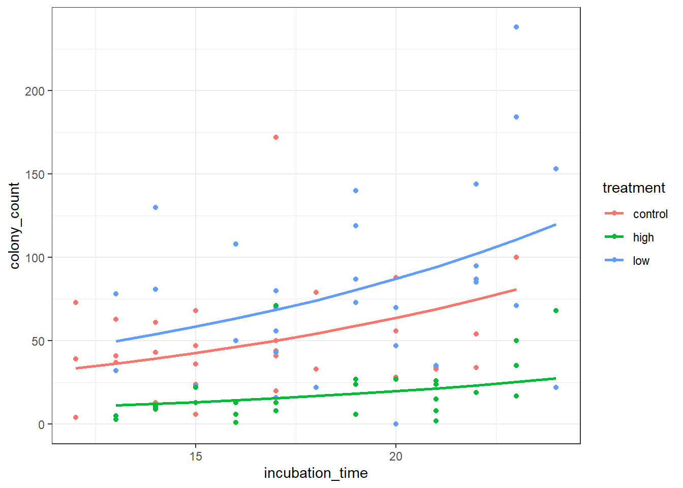

Here’s a more efficient way of doing exactly the same thing - we put the augmented object in directly as our data, and do the exponentiation inside the geom_line aes function:

ggplot(augment(nb_petri), aes(y = colony_count, x = incubation_time, colour = treatment)) +
  geom_point() +
  geom_line(mapping = aes(y = exp(.fitted)), linewidth = 1)

Notice how this is subtly different from the model we would’ve visualised, if we’d just used geom_smooth:

ggplot(petri_aug, aes(y = colony_count, x = incubation_time, colour = treatment)) +
  geom_point() +
  geom_smooth(method = "glm.nb", se = FALSE) +
  labs(title = "This is not the model we wanted!")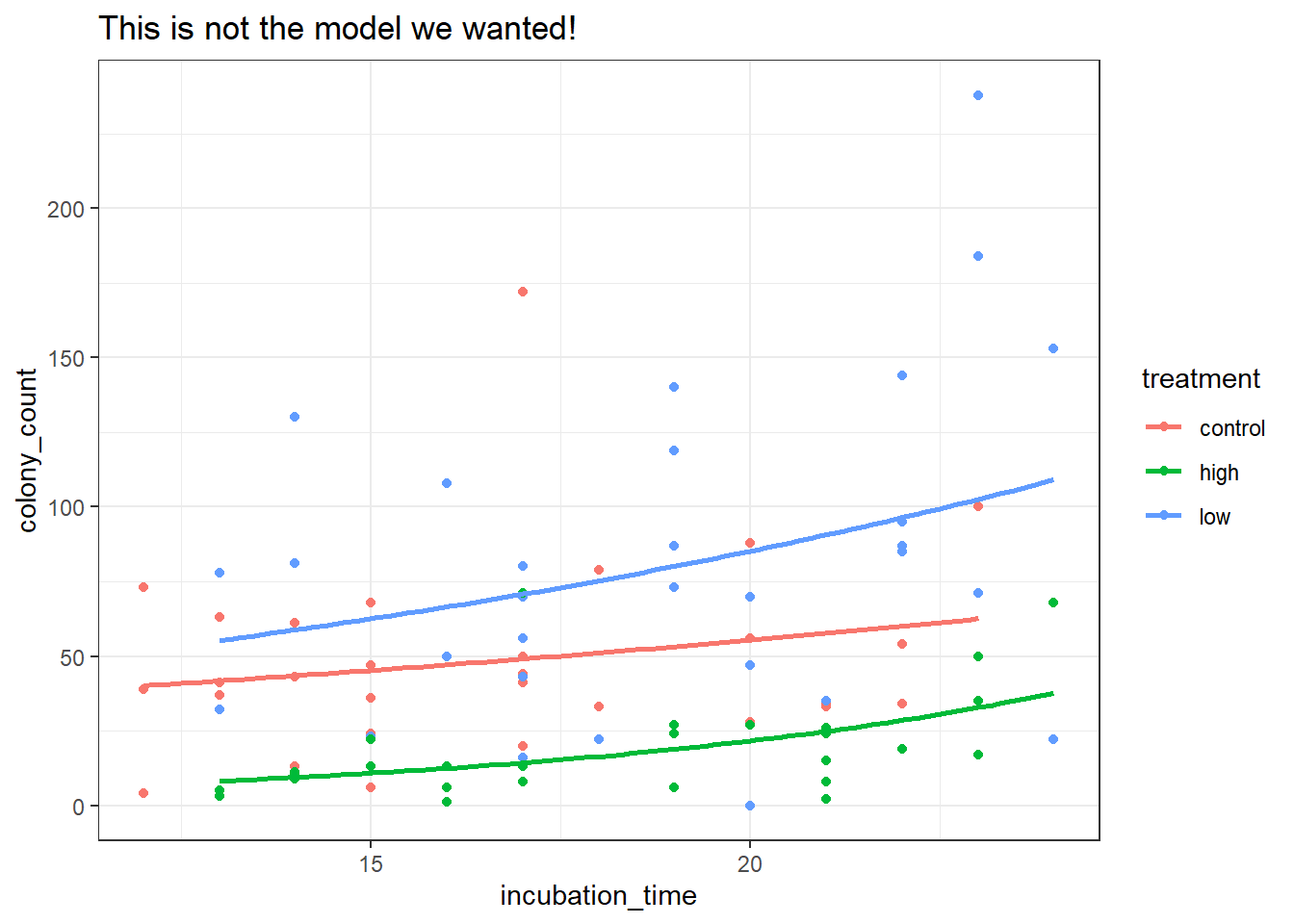

We can copy and adapt the code we used for the parasites example in the main body of the chapter - just remember to change all the names!

# Get unique treatment values
treatment_levels = bacteria['treatment'].unique()

# Create prediction grid for each lake
new_data_nb = pd.concat([
    pd.DataFrame({
        'incubation_time': np.linspace(12, 24, 100), # set sensible start & end!
        'treatment': treatment
    }) for treatment in treatment_levels
])

# Repeat the transformations we used when fitting the model
treatment_dummies = pd.get_dummies(new_data_nb['treatment'], drop_first=True)
X_new = pd.concat([new_data_nb['incubation_time'], treatment_dummies], axis=1)
X_new = sm.add_constant(X_new).astype(float)

# Now we can safely predict:
new_data_nb['pred'] = nb_petri.predict(X_new)

new_data_nb.head()

   incubation_time treatment       pred
0        12.000000   control  33.657760
1        12.121212   control  33.984624
2        12.242424   control  34.314663
3        12.363636   control  34.647907
4        12.484848   control  34.984387

(
  ggplot(bacteria,
         aes(x = "incubation_time",
             y = "colony_count",
             colour = "treatment")) +
     geom_point() +
     geom_line(new_data_nb, aes(x = "incubation_time", y = "pred", colour = "treatment"), size = 1)
)

<Figure Size: (640 x 480)>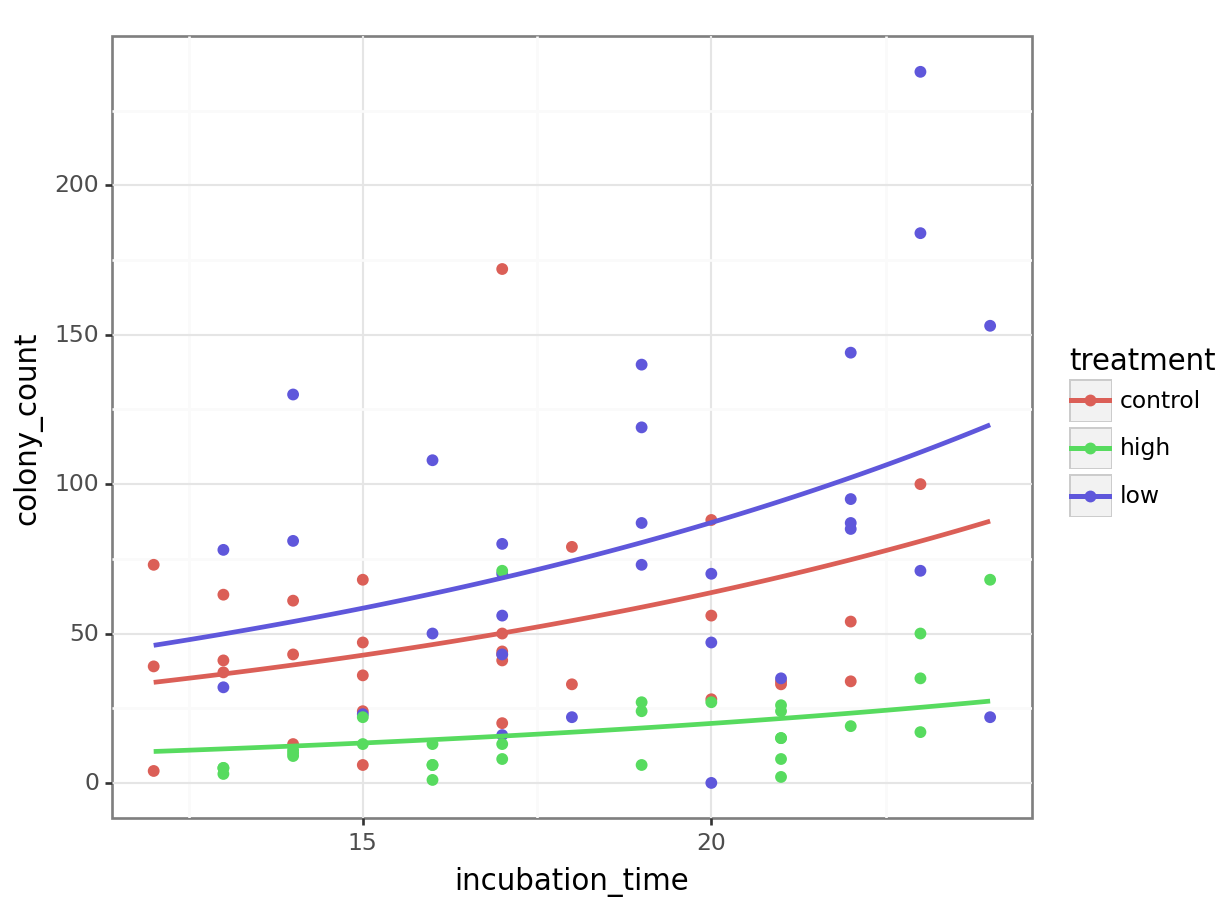

Evaluate assumptions & fit

We don’t need to worry about dispersion - we’re explicitly modelling that, rather than making any assumptions.

We can be reasonably sure we’ve chosen the right response variable distribution and link function; these are clearly count data.

With the info we’ve got, we don’t have any reason to be worried about independence. If, however, we found out more about the design - for example, that the petri dishes had been processed in batches, perhaps by different researchers - that might set off alarm bells.

R
Python

check_model(nb_petri, check = c('pp_check', 'outliers', 'vif'))

Cannot simulate residuals for models of class `negbin`. Please try
  `check_model(..., residual_type = "normal")` instead.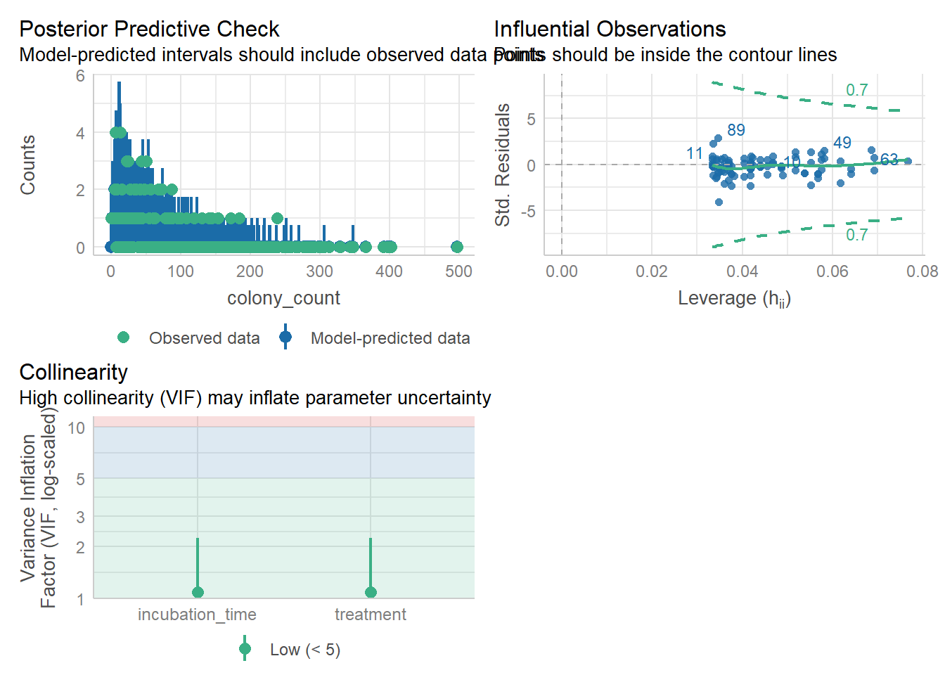

check_collinearity(nb_petri)

# Check for Multicollinearity

Low Correlation

            Term  VIF   VIF 95% CI Increased SE Tolerance Tolerance 95% CI
       treatment 1.08 [1.01, 2.25]         1.04      0.92     [0.44, 0.99]
 incubation_time 1.08 [1.01, 2.25]         1.04      0.92     [0.44, 0.99]

check_outliers(nb_petri, threshold = list('cook'=0.5))

OK: No outliers detected.
- Based on the following method and threshold: cook (0.5).
- For variable: (Whole model)

No obvious issues to report!

Refit the model with smf.glm, so we can access get_influence. Don’t forget to include the estimated alpha.

alpha_est = nb_petri.params['alpha']

model = smf.glm(formula='colony_count ~ treatment + incubation_time',
                data=bacteria,
                family=sm.families.NegativeBinomial(alpha = alpha_est))

glm_nb_petri = model.fit()

Now we can check influential points:

influence = glm_nb_petri.get_influence()

cooks = influence.cooks_distance[0]

influential_points = np.where(cooks > 0.5)[0] # Set appropriate threshold here

print("Influential points:", influential_points)

Influential points: [88]

We have one possible influential point; if this were a real analysis, we would want to follow up on this now, e.g., removing it and refitting, and seeing if our model shifts dramatically.

(Spoiler alert - it doesn’t!)

Collinearity/variance inflation factors:

# Drop the response variable
X = bacteria.drop(columns='colony_count')

# Create design matrix based on model formula
X = dmatrix("treatment + incubation_time", data=bacteria, return_type='dataframe')

# Calculate VIF for each feature
vif_data = pd.DataFrame()
vif_data['feature'] = X.columns
vif_data['VIF'] = [variance_inflation_factor(X.values, i)
                   for i in range(X.shape[1])]

print(vif_data)

             feature        VIF
0          Intercept  28.462829
1  treatment[T.high]   1.379350
2   treatment[T.low]   1.435343
3    incubation_time   1.079513

No issues with the VIF values!

Compare model to null

R
Python

nb_petri_null <- glm.nb(colony_count ~ 1, bacteria)

anova(nb_petri, nb_petri_null)

Likelihood ratio tests of Negative Binomial Models

Response: colony_count
                        Model    theta Resid. df    2 x log-lik.   Test    df
1                           1 1.220838        89       -882.5434             
2 treatment + incubation_time 2.196271        86       -826.6210 1 vs 2     3
  LR stat.      Pr(Chi)
1                      
2 55.92243 4.364176e-12

We’ve not constructed a null model yet earlier in this chapter, so don’t worry if you didn’t figure this bit out on your own.

We still need to set up a Y response and an X predictor matrix. However, since we only want to regress colony_count ~ 1, our X matrix just needs to be a column of 1s, with the same length as Y.

We can set that up like this:

Y = bacteria['colony_count']
X = np.ones((len(Y), 1))

From here, the model fitting proceeds exactly as before.

model = NegativeBinomial(Y, X)

nb_petri_null = model.fit()

Optimization terminated successfully.
         Current function value: 4.903019
         Iterations: 6
         Function evaluations: 7
         Gradient evaluations: 7

nb_petri_null.summary()

NegativeBinomial Regression Results
Dep. Variable:	colony_count	No. Observations:	90
Model:	NegativeBinomial	Df Residuals:	89
Method:	MLE	Df Model:	0
Date:	Thu, 10 Jul 2025	Pseudo R-squ.:	3.732e-12
Time:	13:49:12	Log-Likelihood:	-441.27
converged:	True	LL-Null:	-441.27
Covariance Type:	nonrobust	LLR p-value:	nan

	coef	std err	z	P>\|z\|	[0.025	0.975]
const	3.9035	0.097	40.423	0.000	3.714	4.093
alpha	0.8191	0.116	7.049	0.000	0.591	1.047

We can see that the model, indeed, only contains a constant (intercept) with no predictors. That’s what we wanted.

Now, we want to compare the two models (nb_petri and nb_petri_null). This reuses the likelihood ratio test code we’ve been using so far in the course:

lrstat = -2*(nb_petri_null.llf - nb_petri.llf)

pvalue = chi2.sf(lrstat, nb_petri_null.df_resid - nb_petri.df_resid)

print(lrstat, pvalue)

55.92242554562051 4.364156630704114e-12

In conclusion: our additive model is significant over the null, and there are no glaring concerns with assumptions that are not met.

Our visualisation of the model seems sensible too. The number of colonies increases with incubation time - this seems very plausible - and the high antibacterial condition definitely is stunted compared to the control, as we might expect.

Why does the low antibacterial dose condition seem to have more growth than the control? Well, this could just be a fluke. If we repeated the experiment the effect might vanish.

Or, it might be an indication of a stress-induced growth response in those dishes (i.e., a small amount of antibacterial treatment reveals some sort of resistance).

13.7.2 Galapagos models

Exercise

Level:

For this exercise we’ll be using the data from data/galapagos.csv.

In this dataset, each row corresponds to one of the 30 Galapagos islands. The relationship between the number of plant species (species) and several geographic variables is of interest:

endemics – the number of endemic species
area – the area of the island km²
elevation – the highest elevation of the island (m)
nearest – the distance from the nearest island (km)

However, fitting both a Poisson and a negative binomial regression produce quite bad results, with strange fit.

In this exercise, you should:

Fit and visualise a Poisson model
Fit and visualise a negative binomial model
Explore ways to improve the fit of the model

(Hint: just because we’re fitting a GLM, doesn’t mean we can’t still transform our data!)

A note for Python users

Due to the small (near-zero) beta coefficients for these data, the NegativeBinomial method we’ve been using struggles to converge on a successful model. Therefore, there is no Python code provided for this example.

However, you might find it useful to read through the answer regardless - this is a very interesting dataset!

Answer

galapagos <- read_csv("data/galapagos.csv")

Fitting a Poisson model

glm_gal <- glm(species ~ area + endemics + elevation + nearest,
               data = galapagos, family = "poisson")

p1 <- ggplot(galapagos, aes(endemics, species)) +
  geom_point() +
  geom_smooth(method = "glm", se = FALSE, fullrange = TRUE, 
              method.args = list(family = "poisson")) +
  labs(title = "Poisson")

p1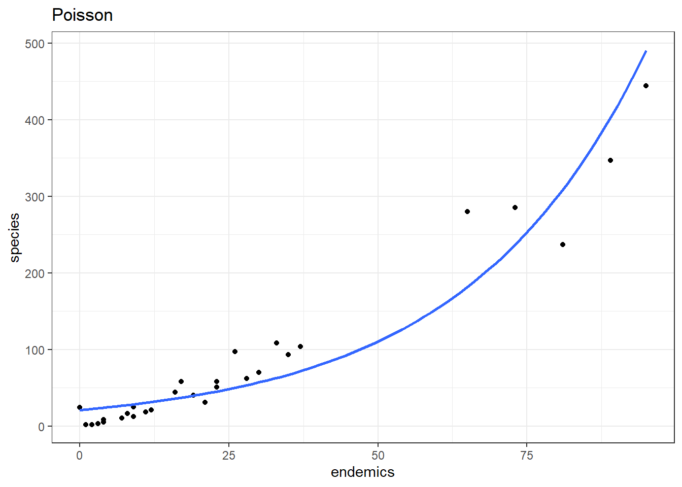

Our model is doing okay over on the right hand side, but it’s not really doing a good job in the bottom left corner - which is where most of the data points are clustered!

Fitting a negative binomial model

nb_gal <- glm.nb(species ~ area + endemics + elevation + nearest,
               data = galapagos)

p2 <- ggplot(galapagos, aes(endemics, species)) +
  geom_point() +
  geom_smooth(method = "glm.nb", se = FALSE, fullrange = TRUE) +
  labs(title = "Negative binomial")

p2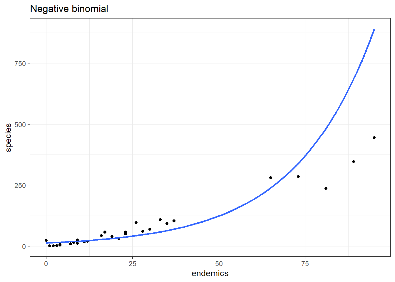

This model does a better job in the lower left, but now is getting things a bit wrong over on the far right.

Improving the fit

Is there anything we can do to improve on these two models?

There appears to be a power relationship between species and endemics. So, one thing we could do is log-transform the response (species) and predictor (endemics) variables.

If we log-transform them both and put them on a scatterplot, they look like this - linear?!

ggplot(data = galapagos,
       aes(x = log(endemics),
           y = log(species))) +
  geom_point()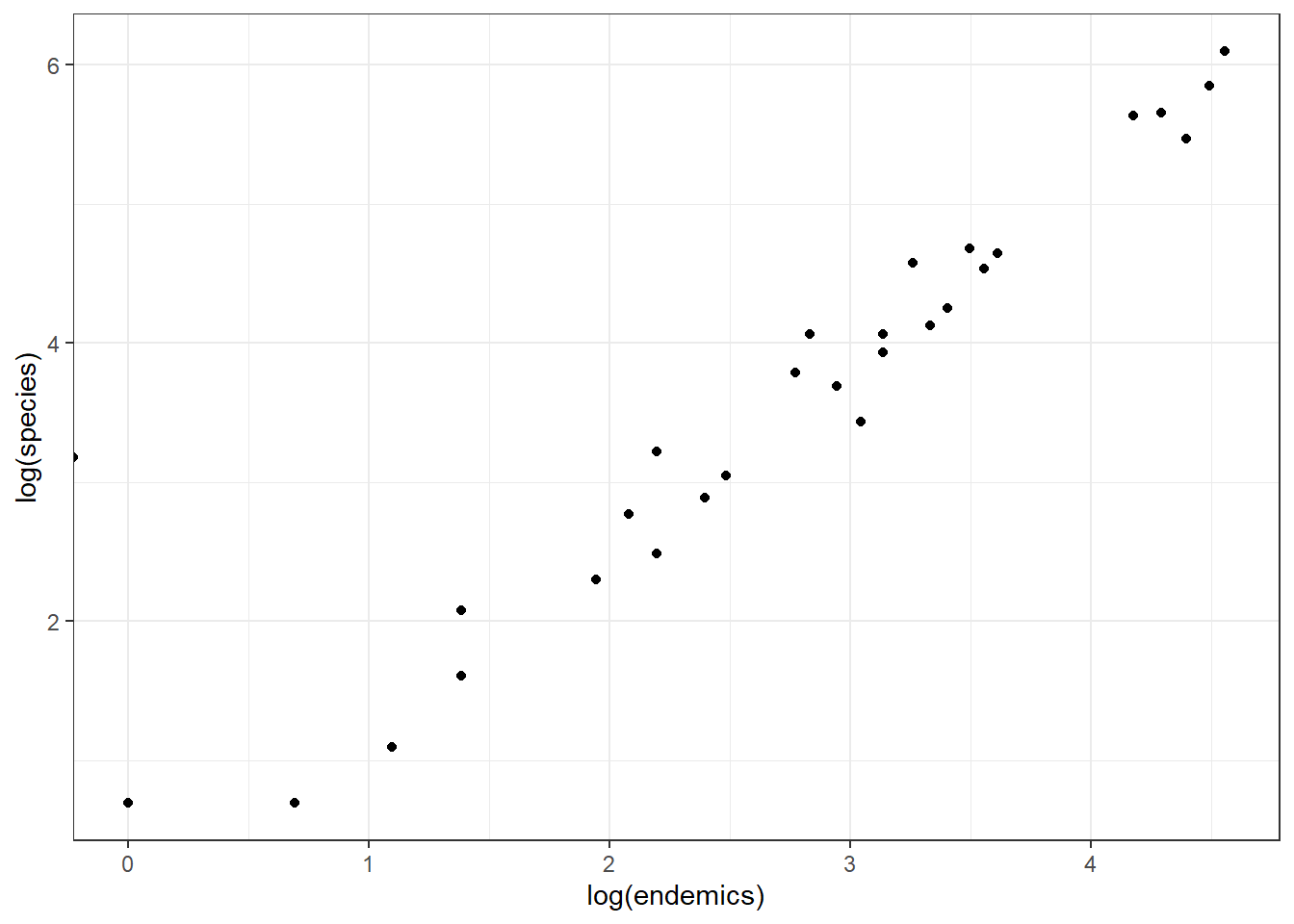

We could add a regression line to this.

Or, we could just log-transform endemics and fit a negative binomial model to that, without also log-transforming species. Let’s do all of this and plot them together with the original Poisson and Negative binomial models.

p3 <- ggplot(galapagos, aes(log(endemics), log(species))) +
  geom_point() +
  geom_smooth(method = "lm", se = FALSE, fullrange = TRUE,
              method.args = list(family = poisson)) +
  labs(title = "Linear model of log-log")

p4 <- ggplot(galapagos, aes(log(endemics), species)) +
  geom_point() +
  geom_smooth(method = "glm.nb", se = FALSE, fullrange = TRUE) +
  ylim(0, 500) +
  labs(title = "Negative binomial of log(endemics)")

library(patchwork)

p1 + p2 + p3 + p4 +
  plot_annotation(tag_levels = "A")

Warning: Removed 1 row containing non-finite outside the scale range
(`stat_smooth()`).

Warning: In lm.wfit(x, y, w, offset = offset, singular.ok = singular.ok, 
    ...) :
 extra argument 'family' will be disregarded

Warning: Removed 1 row containing non-finite outside the scale range
(`stat_smooth()`).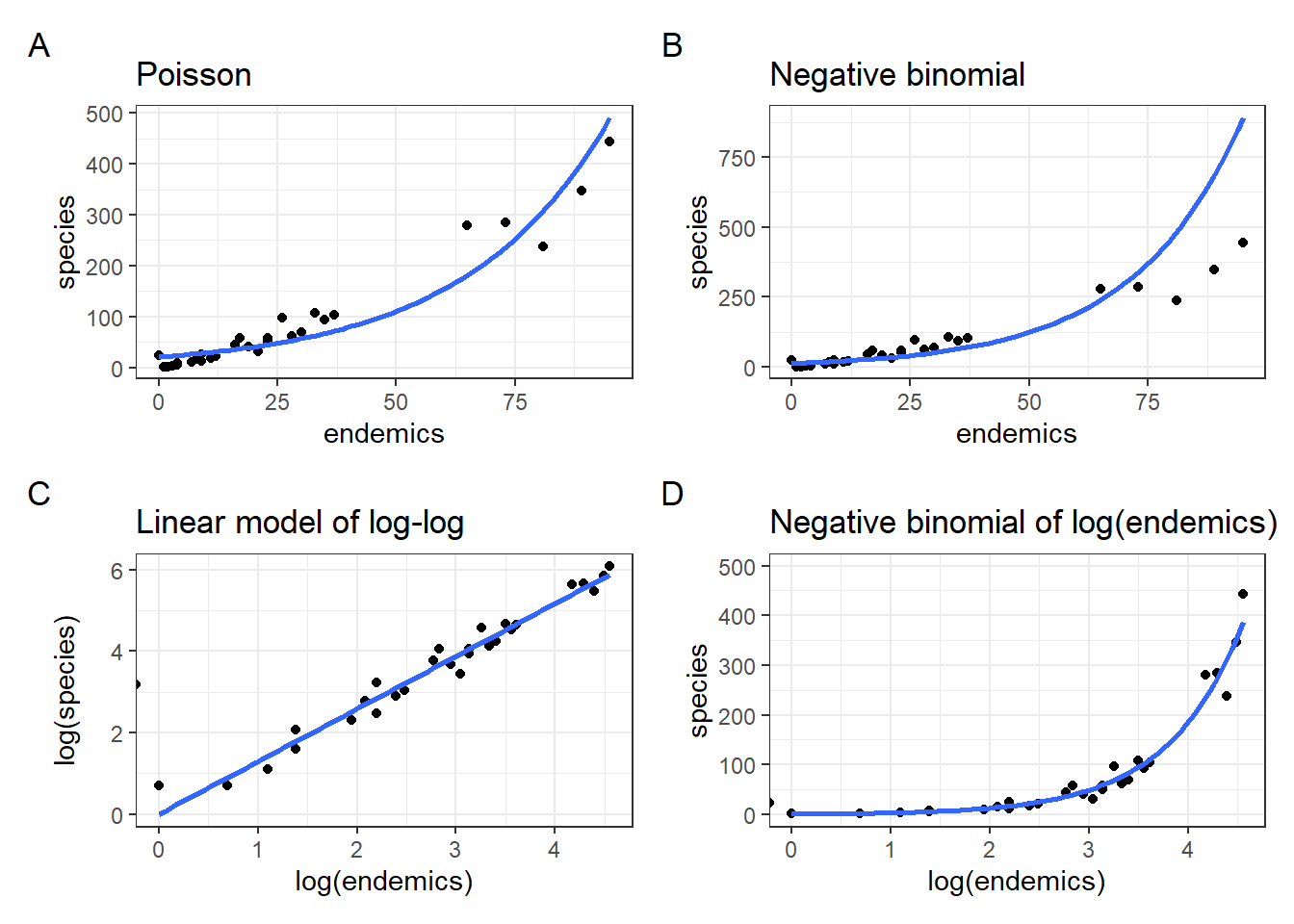

From this it is clear that the negative binomial model fitted to species ~ log(endemics) in panel D produces a much better fit than the original fit in panel B.

Equally, looking at the relationship between log(species) ~ log(endemics) in panel C it illustrates that this is pretty well-modelled using a linear line.

There is a slight issue, though.

If you look carefully then you see that in both panels C and D there is a stray value left of zero, almost escaping past the y-axis. There is also a warning message, saying Removed 1 row containing non-finite outside the scale range.

With a closer look at the dataset, we can see that there is one island where the number of endemics is equal to 0:

galapagos %>% 
  arrange(endemics) %>%
  head(1)

# A tibble: 1 × 5
  species endemics  area elevation nearest
    <dbl>    <dbl> <dbl>     <dbl>   <dbl>
1      24        0  0.08        93       6

If we take log(0) we get minus infinity, which isn’t biologically possible. This is where the problem lies.

We could adjust for this by adding a “pseudo-count”, or adding 1 to all of the counts. If that is acceptable or not is a matter of debate and we’ll leave it to you to ponder over this.

Whatever you do, the most important thing is to make sure that you are transparent and clear on what you are doing and what the justification for it it.

13.8 Summary

Key points

Negative binomial regression relaxes the assumption made by Poisson regressions that the variance is equal to the mean (dispersion = 1)
In a negative binomial regression the dispersion parameter \(\theta\) is estimated from the data
However, they both use the log link function and often produce similar-looking models