12 Analysing count data

Learning outcomes

Questions

How do we analyse count data?

Objectives

Be able to perform a poisson regression on count data

12.1 Libraries and functions

Click to expand

R
Python

12.1.1 Libraries

library(ggResidpanel)
library(tidyverse)

12.1.2 Functions

# create diagnostic plots
ggResidpanel::resid_panel()

12.1.3 Libraries

# A maths library
import math
# A Python data analysis and manipulation tool
import pandas as pd

# Python equivalent of `ggplot2`
from plotnine import *

# Statistical models, conducting tests and statistical data exploration
import statsmodels.api as sm

# Convenience interface for specifying models using formula strings and DataFrames
import statsmodels.formula.api as smf

# Needed for additional probability functionality
from scipy.stats import *

12.1.4 Functions

The examples in this section use the following data sets:

data/islands.csv

This is a data set comprising 35 observations of two variables (one dependent and one predictor). This records the number of species recorded on different small islands along with the area (km²) of the islands. The variables are species and area.

The second data set is on seat belts.

The seatbelts data set is a multiple time-series data set that was commissioned by the Department of Transport in 1984 to measure differences in deaths before and after front seat belt legislation was introduced on 31st January 1983. It provides monthly total numerical data on a number of incidents including those related to death and injury in Road Traffic Accidents (RTA’s). The data set starts in January 1969 and observations run until December 1984.

You can find the file in data/seatbelts.csv

12.2 Load and visualise the data

First we load the data, then we visualise it.

R
Python

islands <- read_csv("data/islands.csv")

Let’s have a glimpse at the data:

islands

# A tibble: 35 × 2
   species  area
     <dbl> <dbl>
 1     114  12.1
 2     130  13.4
 3     113  13.7
 4     109  14.5
 5     118  16.8
 6     136  19.0
 7     149  19.6
 8     162  20.6
 9     145  20.9
10     148  21.0
# ℹ 25 more rows

islands_py = pd.read_csv("data/islands.csv")

Let’s have a glimpse at the data:

islands_py.head()

   species       area
0      114  12.076133
1      130  13.405439
2      113  13.723525
3      109  14.540359
4      118  16.792122

Looking at the data, we can see that there are two columns: species, which contains the number of species recorded on each island and area, which contains the surface area of the island in square kilometers.

We can plot the data:

R
Python

ggplot(islands, aes(x = area, y = species)) +
  geom_point()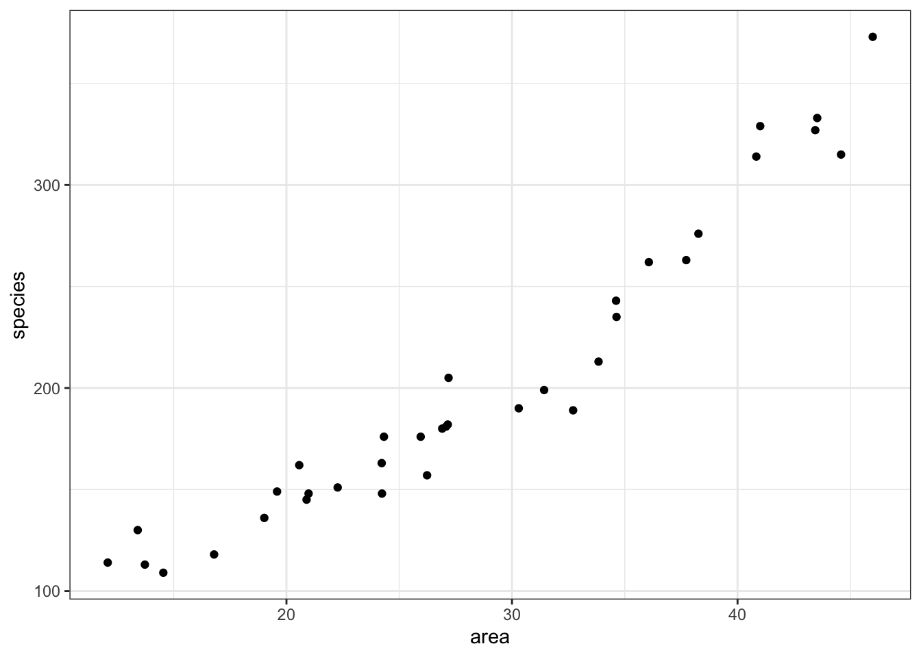

Figure 12.1: Scatterplot of area and species

(ggplot(islands_py, aes(x = "area", y = "species")) +
  geom_point())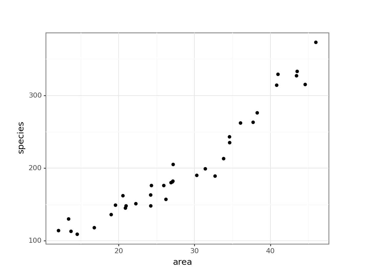

Figure 12.2: Scatterplot of area and species

It looks as though area may have an effect on the number of species that we observe on each island. We note that the response variable is count data and so we try to construct a Poisson regression.

glm_isl <- glm(species ~ area,
               data = islands, family = "poisson")

and we look at the model summary:

summary(glm_isl)


Call:
glm(formula = species ~ area, family = "poisson", data = islands)

Coefficients:
            Estimate Std. Error z value Pr(>|z|)    
(Intercept) 4.241129   0.041322  102.64   <2e-16 ***
area        0.035613   0.001247   28.55   <2e-16 ***
---
Signif. codes:  0 '***' 0.001 '**' 0.01 '*' 0.05 '.' 0.1 ' ' 1

(Dispersion parameter for poisson family taken to be 1)

    Null deviance: 856.899  on 34  degrees of freedom
Residual deviance:  30.437  on 33  degrees of freedom
AIC: 282.66

Number of Fisher Scoring iterations: 3

The output is strikingly similar to the logistic regression models (who’d have guessed, eh?) and the main numbers to extract from the output are the two numbers underneath Estimate.Std in the Coefficients table:

(Intercept)    4.241129
area           0.035613

# create a generalised linear model
model = smf.glm(formula = "species ~ area",
                family = sm.families.Poisson(),
                data = islands_py)
# and get the fitted parameters of the model
glm_isl_py = model.fit()

Let’s look at the model output:

print(glm_isl_py.summary())

                 Generalized Linear Model Regression Results                  
==============================================================================
Dep. Variable:                species   No. Observations:                   35
Model:                            GLM   Df Residuals:                       33
Model Family:                 Poisson   Df Model:                            1
Link Function:                    Log   Scale:                          1.0000
Method:                          IRLS   Log-Likelihood:                -139.33
Date:                Fri, 14 Jun 2024   Deviance:                       30.437
Time:                        13:05:13   Pearson chi2:                     30.3
No. Iterations:                     4   Pseudo R-squ. (CS):              1.000
Covariance Type:            nonrobust                                         
==============================================================================
                 coef    std err          z      P>|z|      [0.025      0.975]
------------------------------------------------------------------------------
Intercept      4.2411      0.041    102.636      0.000       4.160       4.322
area           0.0356      0.001     28.551      0.000       0.033       0.038
==============================================================================

These are the coefficients of the Poisson model equation and need to be placed in the following formula in order to estimate the expected number of species as a function of island size:

\[ E(species) = \exp(4.24 + 0.036 \times area) \]

Interpreting this requires a bit of thought (not much, but a bit). The intercept coefficient, 4.24, is related to the number of species we would expect on an island of zero area (this is statistics, not real life. You’d do well to remember that before you worry too much about what that even means). But in order to turn this number into something meaningful we have to exponentiate it. Since exp(4.24) ≈ 70, we can say that the baseline number of species the model expects on any island is 70. This isn’t actually the interesting bit though.

The coefficient of area is the fun bit. For starters we can see that it is a positive number which does mean that increasing area leads to increasing numbers of species. Good so far.

But what does the value 0.036 actually mean? Well, if we exponentiate it as well, we get exp(0.036) ≈ 1.04. This means that for every increase in area of 1 km² (the original units of the area variable), the number of species on the island is multiplied by 1.04. So, an island of area km² will have \(1.04 \times 70 \approx 72\) species.

So, in order to interpret Poisson coefficients, you have to exponentiate them.

12.4 Plotting the Poisson regression

R
Python

ggplot(islands, aes(area, species)) +
  geom_point() +
  geom_smooth(method = "glm", se = FALSE, fullrange = TRUE, 
              method.args = list(family = "poisson")) +
  xlim(10,50)

`geom_smooth()` using formula = 'y ~ x'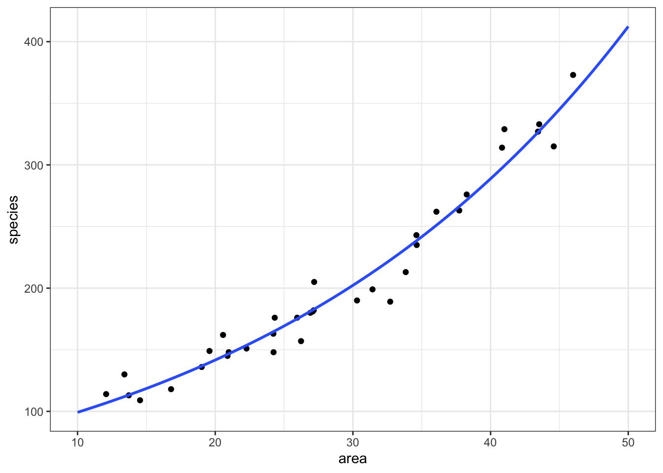

Figure 12.3: Poisson regression on species ~ area

model = pd.DataFrame({'area': list(range(10, 50))})

model["pred"] = glm_isl_py.predict(model)

model.head()

   area        pred
0    10   99.212463
1    11  102.809432
2    12  106.536811
3    13  110.399326
4    14  114.401877

(ggplot(islands_py,
         aes(x = "area",
             y = "species")) +
     geom_point() +
     geom_line(model, aes(x = "area", y = "pred"), colour = "blue", size = 1))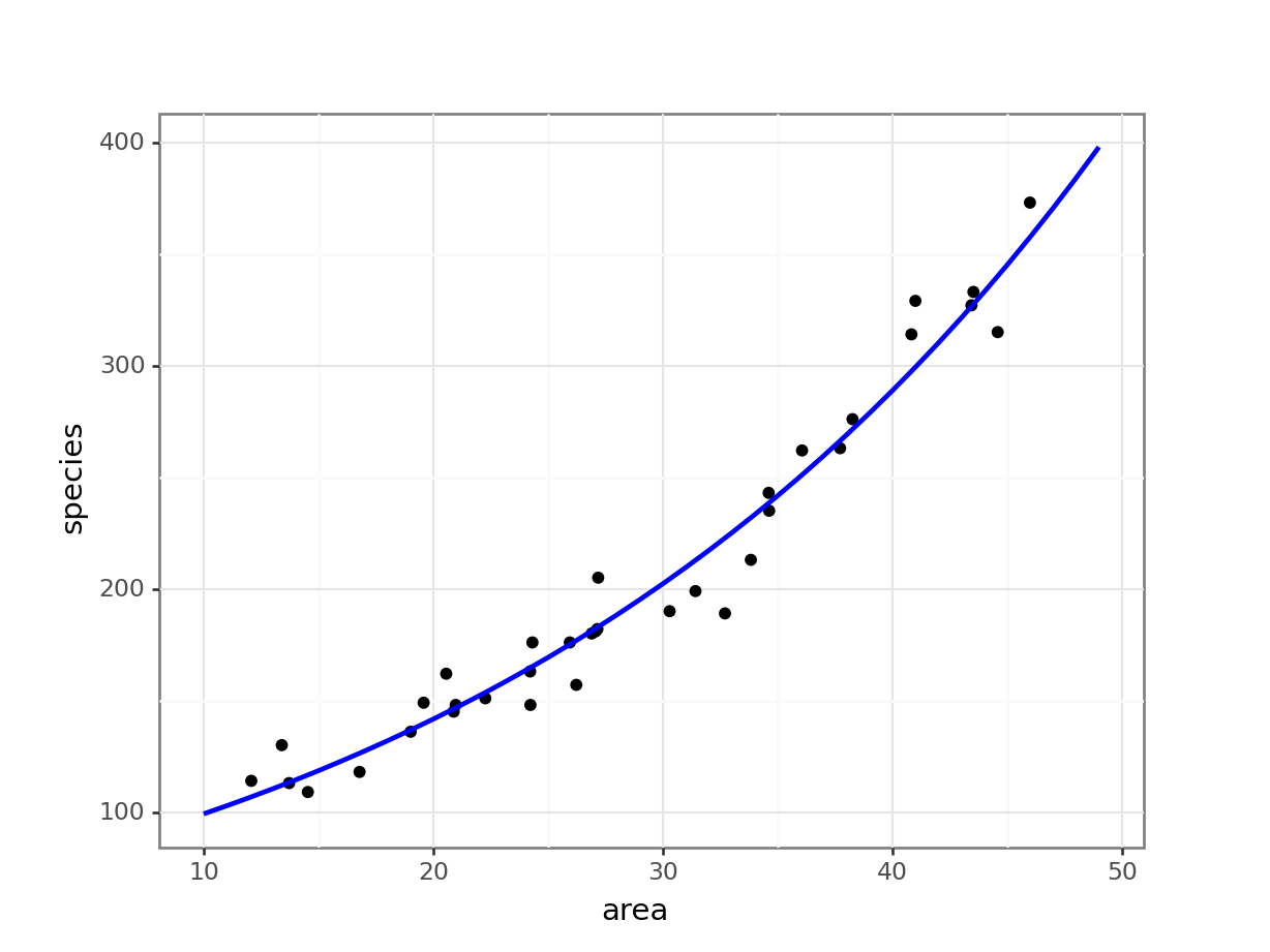

Figure 12.4: Poisson regression on species ~ area

12.5 Assumptions

As we mentioned earlier, Poisson regressions require that the variance of the data at any point is the same as the mean of the data at that point. We checked that earlier by looking at the residual deviance values.

We can look for influential points using the Cook’s distance plot:

R
Python

resid_panel(glm_isl, plots = c("cookd"))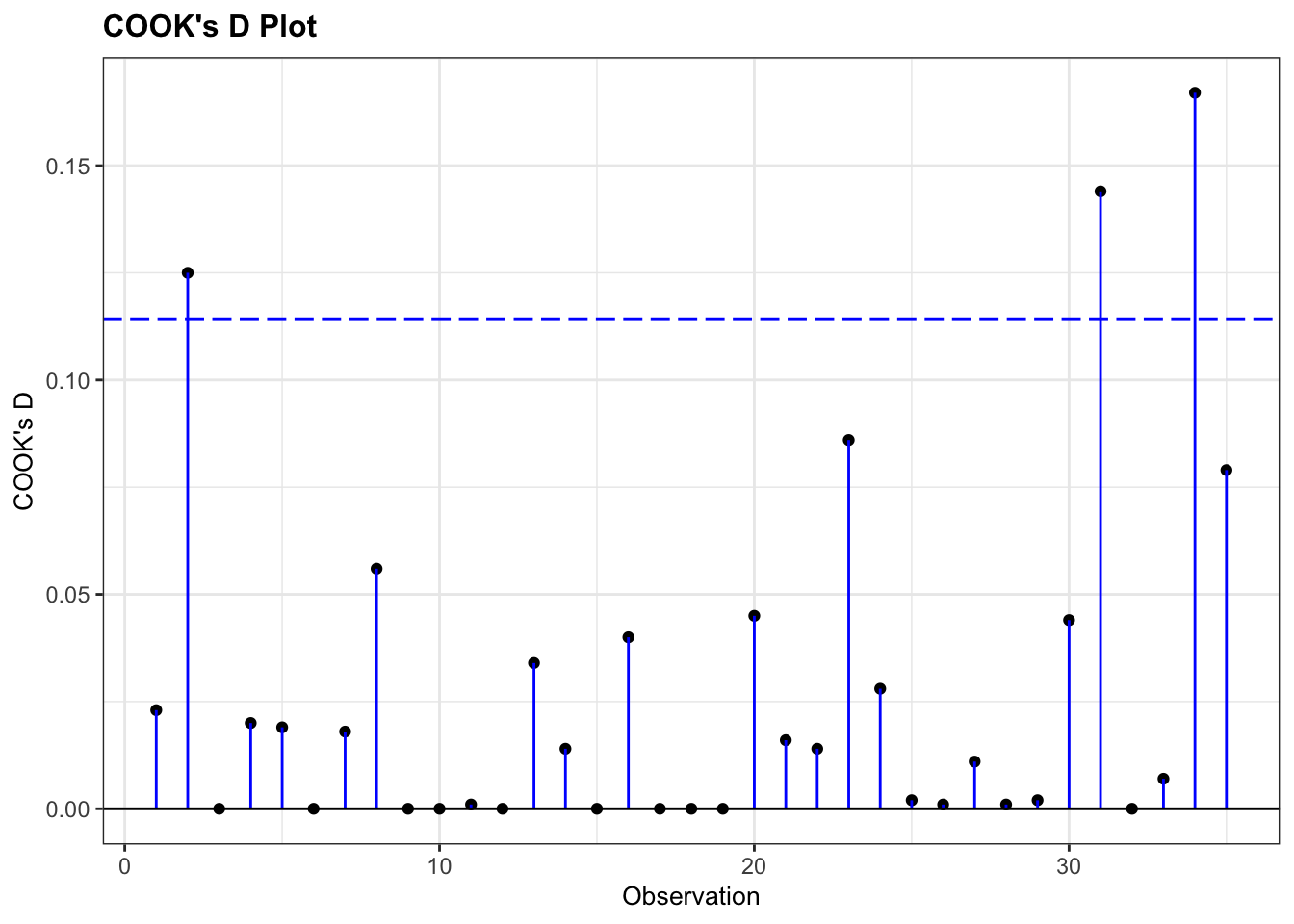

# extract the Cook's distances
glm_isl_py_resid = pd.DataFrame(glm_isl_py.
                                get_influence().
                                summary_frame()["cooks_d"])

# add row index 
glm_isl_py_resid['obs'] = glm_isl_py_resid.reset_index().index

We can use these to create the plot:

(ggplot(glm_isl_py_resid,
         aes(x = "obs",
             y = "cooks_d")) +
     geom_segment(aes(x = "obs", y = "cooks_d", xend = "obs", yend = 0)) +
     geom_point())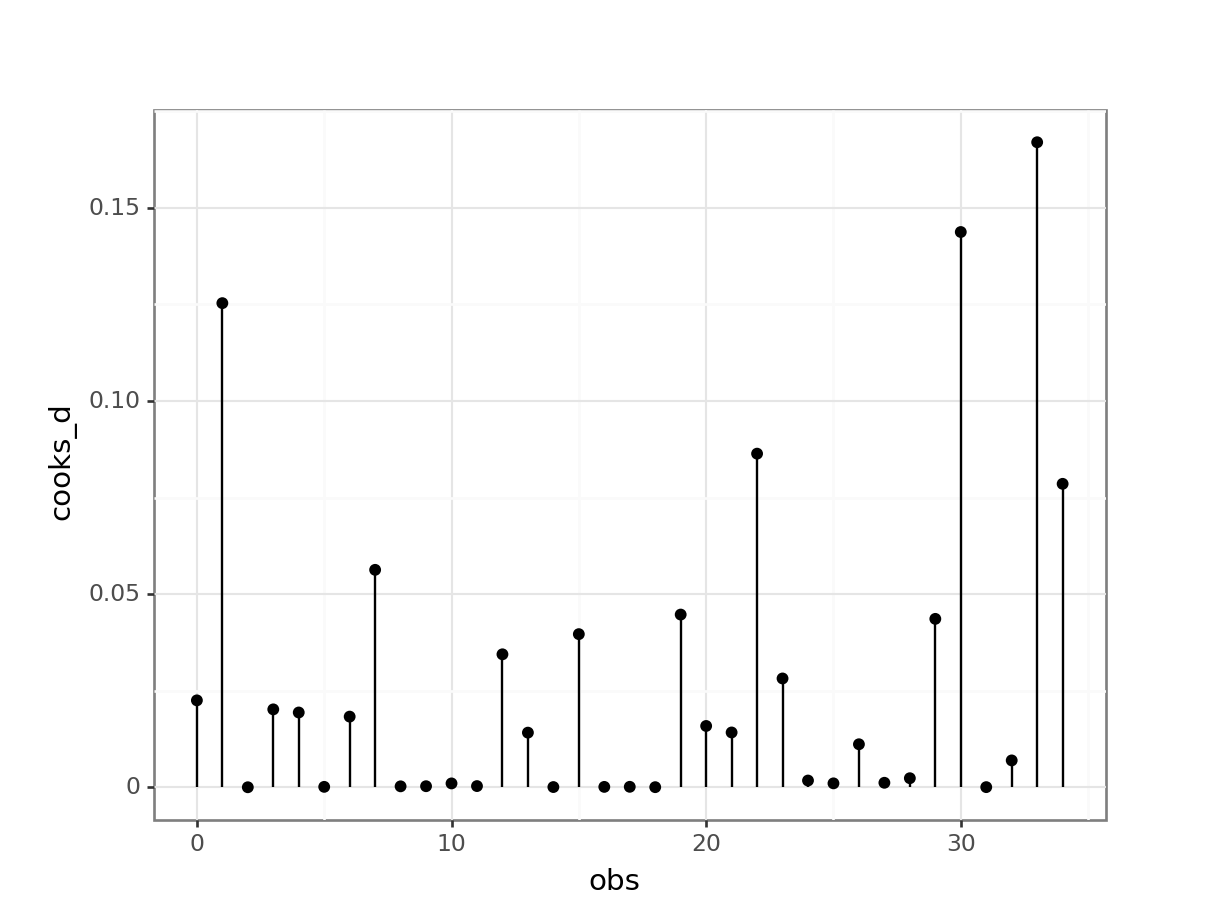

None of our points have particularly large Cook’s distances and so life is rosy.

12.6 Assessing significance

We can ask the same three questions we asked before.

Is the model well-specified?
Is the overall model better than the null model?
Are any of the individual predictors significant?

Again, in this case, questions 2 and 3 are effectively asking the same thing because we still only have a single predictor variable.

To assess if the model is any good we’ll again use the residual deviance and the residual degrees of freedom.

R
Python

1 - pchisq(30.437, 33)

[1] 0.5953482

chi2.sf(30.437, 33)

0.5953481872979622

This gives a probability of 0.60. This suggests that this model is actually a reasonably decent one and that the data are pretty well supported by the model. For Poisson models this has an extra interpretation. This can be used to assess whether we have significant over-dispersion in our data.

For a Poisson model to be appropriate we need that the variance of the data to be exactly the same as the mean of the data. Visually, this would correspond to the data spreading out more for higher predicted values of species. However, we don’t want the data to spread out too much. If that happens then a Poisson model wouldn’t be appropriate.

The easy way to check this is to look at the ratio of the residual deviance to the residual degrees of freedom (in this case 0.922). For a Poisson model to be valid, this ratio should be about 1. If the ratio is significantly bigger than 1 then we say that we have over-dispersion in the model and we wouldn’t be able to trust any of the significance testing that we are about to do using a Poisson regression.

Thankfully the probability we have just created (0.60) is exactly the right one we need to look at to assess whether we have significant over-dispersion in our model.

Secondly, to assess whether the overall model, with all of the terms, is better than the null model we’ll look at the difference in deviances and the difference in degrees of freedom:

R
Python

1 - pchisq(856.899 - 30.437, 34 - 33)

[1] 0

chi2.sf(856.899 - 30.437, 34 - 33)

9.524927068555617e-182

This gives a reported p-value of pretty much zero, which is rather small. So, yes, this model is better than nothing at all and species does appear to change with some of our predictors

Finally, we’ll construct an analysis of deviance table to look at the individual terms:

R
Python

anova(glm_isl , test = "Chisq")

Analysis of Deviance Table

Model: poisson, link: log

Response: species

Terms added sequentially (first to last)

     Df Deviance Resid. Df Resid. Dev  Pr(>Chi)    
NULL                    34     856.90              
area  1   826.46        33      30.44 < 2.2e-16 ***
---
Signif. codes:  0 '***' 0.001 '**' 0.01 '*' 0.05 '.' 0.1 ' ' 1

The p-value in this table is just as small as we’d expect given our previous result (<2.2e-16 is pretty close to 0), and we have the nice consistent result that area definitely has an effect on species.

As mentioned before, this is not quite possible in Python.

12.7 Exercises

12.7.1 Seat belts

Exercise

Level:

For this exercise we’ll be using the data from data/seatbelts.csv.

I’d like you to do the following:

Load the data
Visualise the data and create a poisson regression model
Plot the regression model on top of the data
Assess if the model is a decent predictor for the number of fatalities

Answer

Load and visualise the data

First we load the data, then we visualise it.

R
Python

seatbelts <- read_csv("data/seatbelts.csv")

seatbelts_py = pd.read_csv("data/seatbelts.csv")

Let’s have a glimpse at the data:

seatbelts_py.head()

   casualties  drivers  front  rear  ...  van_killed  law  year  month
0         107     1687    867   269  ...          12    0  1969    Jan
1          97     1508    825   265  ...           6    0  1969    Feb
2         102     1507    806   319  ...          12    0  1969    Mar
3          87     1385    814   407  ...           8    0  1969    Apr
4         119     1632    991   454  ...          10    0  1969    May

[5 rows x 10 columns]

The data tracks the number of drivers killed in road traffic accidents, before and after the seat belt law was introduced. The information on whether the law was in place is encoded in the law column as 0 (law not in place) or 1 (law in place).

There are many more observations when the law was not in place, so we need to keep this in mind when we’re interpreting the data.

First we have a look at the data comparing no law vs law:

R
Python

We have to convert the law column to a factor, otherwise R will see it as numerical.

seatbelts %>% 
  ggplot(aes(as_factor(law), casualties)) +
   geom_boxplot()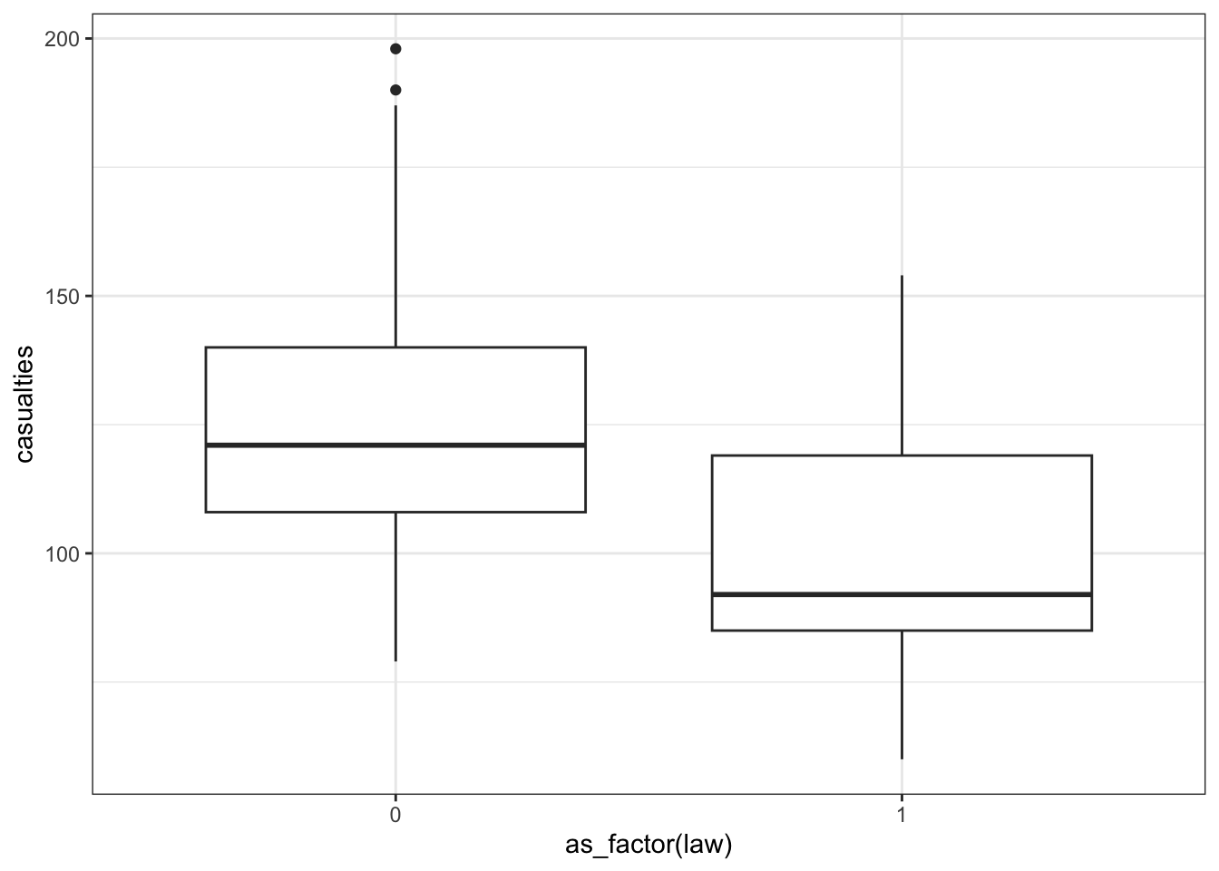

Figure 12.5: Boxplot of driver casualties before and after seatbelt introduction

The data are recorded by month and year, so we can also display the number of drivers killed by year:

seatbelts %>% 
  ggplot(aes(year, casualties)) +
  geom_point()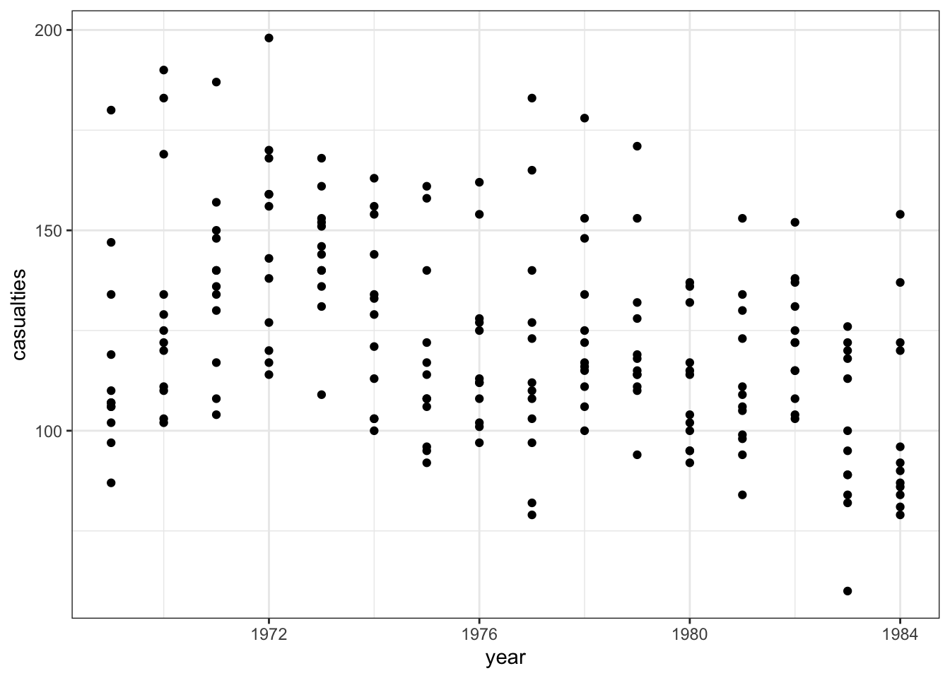

Figure 12.6: Scatterplot of driver casualties across years

We have to convert the law column to a factor, otherwise R will see it as numerical.

(ggplot(seatbelts_py,
         aes(x = seatbelts_py.law.astype(object),
             y = "casualties")) +
     geom_boxplot())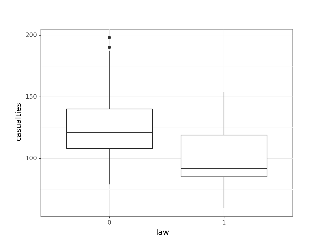

Figure 12.7: Boxplot of driver casualties before and after seatbelt introduction

The data are recorded by month and year, so we can also display the number of casualties by year:

(ggplot(seatbelts_py,
         aes(x = "year",
             y = "casualties")) +
     geom_point())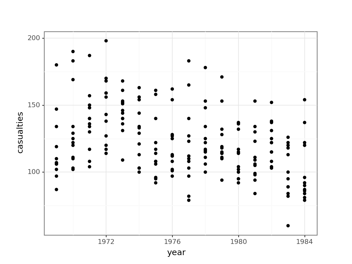

Figure 12.8: Scatterplot of driver casualties across years

The data look a bit weird. There is quite some variation within years (keeping in mind that the data are aggregated monthly). The data also seems to wave around a bit… with some vague peaks (e.g. 1972 - 1973) and some troughs (e.g. around 1976).

So my initial thought is that these data are going to be a bit tricky to interpret. But that’s OK.

Constructing a model

R
Python

glm_stb <- glm(casualties ~ year,
               data = seatbelts, family = "poisson")

and we look at the model summary:

summary(glm_stb)


Call:
glm(formula = casualties ~ year, family = "poisson", data = seatbelts)

Coefficients:
             Estimate Std. Error z value Pr(>|z|)    
(Intercept) 37.168958   2.796636   13.29   <2e-16 ***
year        -0.016373   0.001415  -11.57   <2e-16 ***
---
Signif. codes:  0 '***' 0.001 '**' 0.01 '*' 0.05 '.' 0.1 ' ' 1

(Dispersion parameter for poisson family taken to be 1)

    Null deviance: 984.50  on 191  degrees of freedom
Residual deviance: 850.41  on 190  degrees of freedom
AIC: 2127.2

Number of Fisher Scoring iterations: 4

(Intercept)    37.168958
year           -0.016373

# create a linear model
model = smf.glm(formula = "casualties ~ year",
                family = sm.families.Poisson(),
                data = seatbelts_py)
# and get the fitted parameters of the model
glm_stb_py = model.fit()

print(glm_stb_py.summary())

                 Generalized Linear Model Regression Results                  
==============================================================================
Dep. Variable:             casualties   No. Observations:                  192
Model:                            GLM   Df Residuals:                      190
Model Family:                 Poisson   Df Model:                            1
Link Function:                    Log   Scale:                          1.0000
Method:                          IRLS   Log-Likelihood:                -1061.6
Date:                Fri, 14 Jun 2024   Deviance:                       850.41
Time:                        13:05:15   Pearson chi2:                     862.
No. Iterations:                     4   Pseudo R-squ. (CS):             0.5026
Covariance Type:            nonrobust                                         
==============================================================================
                 coef    std err          z      P>|z|      [0.025      0.975]
------------------------------------------------------------------------------
Intercept     37.1690      2.797     13.291      0.000      31.688      42.650
year          -0.0164      0.001    -11.569      0.000      -0.019      -0.014
==============================================================================

======================
                 coef  
----------------------
Intercept     37.1690 
year          -0.0164 
======================

These are the coefficients of the Poisson model equation and need to be placed in the following formula in order to estimate the expected number of species as a function of island size:

\[ E(casualties) = \exp(37.17 - 0.164 \times year) \]

Assessing significance

Is the model well-specified?

R
Python

1 - pchisq(850.41, 190)

[1] 0

chi2.sf(850.41, 190)

3.1319689119997022e-84

This value indicates that the model is actually pretty bad. Remember that this value gives you a measure for “the probability that this model is good”. In this case, that’s a very low probability.

How about the overall fit, compared to the null model?

R
Python

1 - pchisq(984.50 - 850.41, 191 - 190)

[1] 0

First we need to define the null model:

# create a linear model
model = smf.glm(formula = "casualties ~ 1",
                family = sm.families.Poisson(),
                data = seatbelts_py)
# and get the fitted parameters of the model
glm_stb_null_py = model.fit()

print(glm_stb_null_py.summary())

                 Generalized Linear Model Regression Results                  
==============================================================================
Dep. Variable:             casualties   No. Observations:                  192
Model:                            GLM   Df Residuals:                      191
Model Family:                 Poisson   Df Model:                            0
Link Function:                    Log   Scale:                          1.0000
Method:                          IRLS   Log-Likelihood:                -1128.6
Date:                Fri, 14 Jun 2024   Deviance:                       984.50
Time:                        13:05:15   Pearson chi2:                 1.00e+03
No. Iterations:                     4   Pseudo R-squ. (CS):          1.942e-13
Covariance Type:            nonrobust                                         
==============================================================================
                 coef    std err          z      P>|z|      [0.025      0.975]
------------------------------------------------------------------------------
Intercept      4.8106      0.007    738.670      0.000       4.798       4.823
==============================================================================

chi2.sf(984.50 - 850.41, 191 - 190)

5.2214097202831414e-31

This indicates that the model is at least markedly better than the null model.

Plotting the regression

R
Python

ggplot(seatbelts, aes(year, casualties)) +
  geom_point() +
  geom_smooth(method = "glm", se = FALSE, fullrange = TRUE, 
              method.args = list(family = poisson)) +
  xlim(1970, 1985)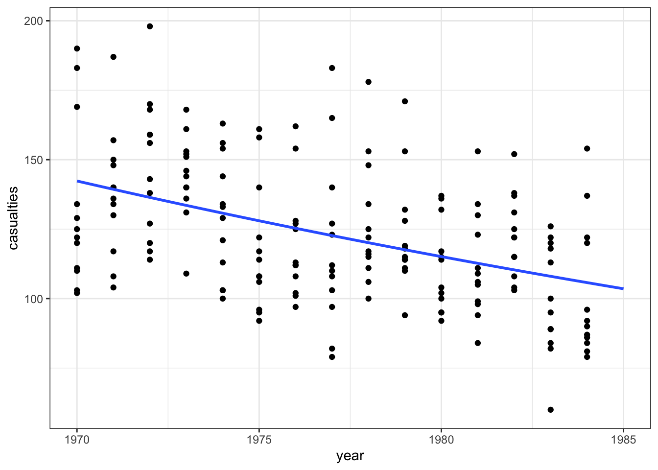

Figure 12.9: Poisson regression of driver casualties across years

model = pd.DataFrame({'year': list(range(1968, 1985))})

model["pred"] = glm_stb_py.predict(model)

model.head()

   year        pred
0  1968  140.737690
1  1969  138.452153
2  1970  136.203733
3  1971  133.991827
4  1972  131.815842

(ggplot(seatbelts_py,
         aes(x = "year",
             y = "casualties")) +
     geom_point() +
     geom_line(model, aes(x = "year", y = "pred"), colour = "blue", size = 1))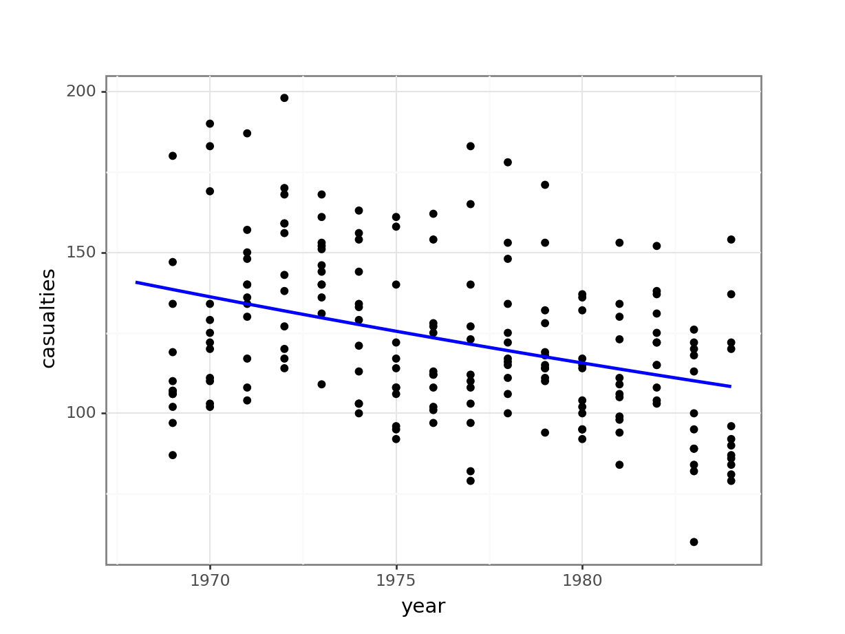

Figure 12.10: Poisson regression of driver casualties across years

Conclusions

Overall, the model we constructed doesn’t seem to be a decent predictor for the number of fatalities.

12.7.2 Seat belts extended

Exercise

Level:

Revisit Exercise 12.7.1, exploring how well the model fits across a wider range of years. Try and answer the following:

Is the model still a good fit?
Do we need to adjust our conclusions?
What improvements to the model can you think of?

12.8 Summary

Key points

Poisson regression is useful when dealing with count data