install.packages("lmtest")
library(lmtest)9 Significance testing
Generalised linear models are fitted a little differently to standard linear models - namely, using maximum likelihood estimation instead of ordinary least squares for estimating the model coefficients.
As a result, we can no longer use F-tests for significance, or interpret \(R^2\) values in quite the same way. This section will discuss new techniques for significance and goodness-of-fit testing, specifically for use with GLMs.
9.1 Libraries and functions
Click to expand
from scipy.stats import *9.2 Deviance
Several of the tests and metrics we’ll discuss below are based heavily on deviance. So, what is deviance, and where does it come from?
Fitting a model using maximum likelihood estimation - the method that we use for GLMs, among other models - is all about finding the parameters that maximise the likelihood, or joint probability, of the sample. In other words, how likely is it that you would sample a set of data points like these, if they were being drawn from an underlying population where your model is true? Each model that you fit has its own likelihood.
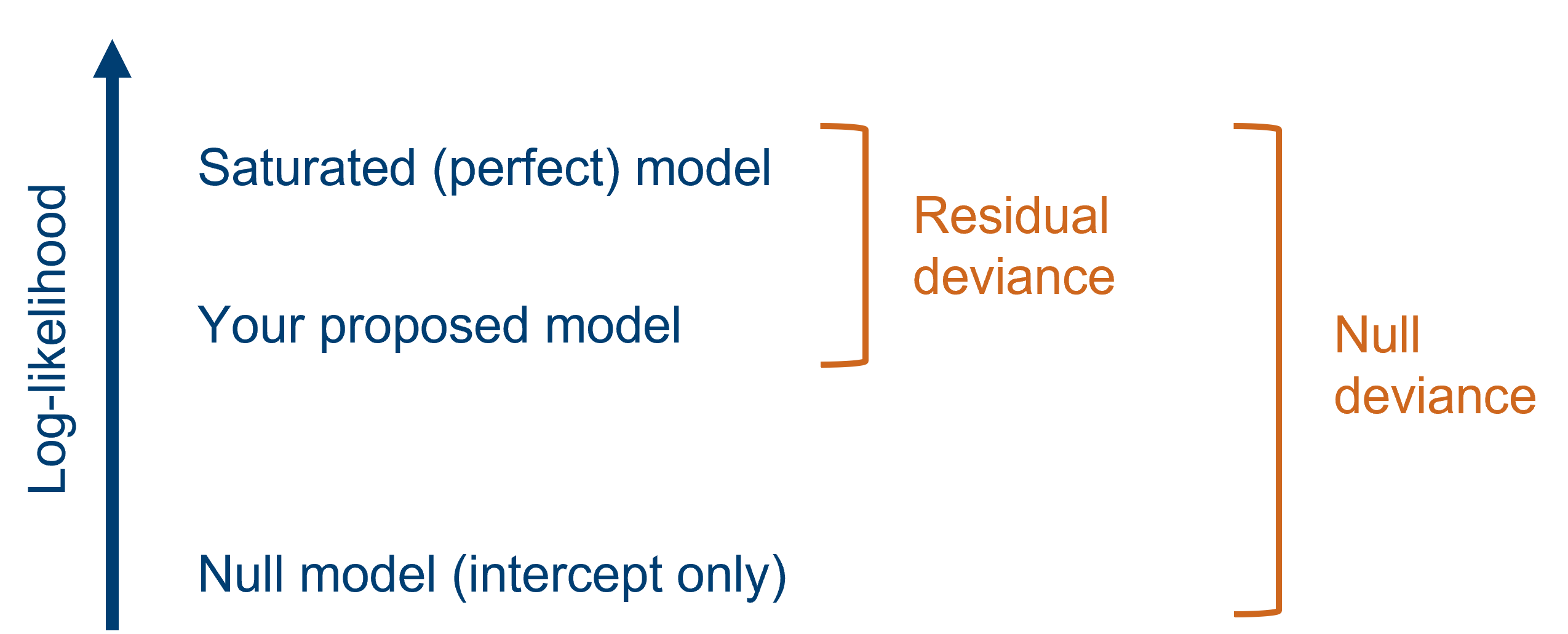
Now, for each dataset, there is a “saturated”, or perfect, model. This model has the same number of parameters in it as there are data points, meaning the data are fitted exactly - as if connecting the dots between them. The saturated model has the largest possible likelihood of any model fitted to the dataset.
Of course, we don’t actually use the saturated model for drawing real conclusions, but we can use it as a baseline for comparison. We compare each model that we fit to this saturated model, to calculate the deviance. Deviance is defined as the difference between the log-likelihood of your fitted model and the log-likelihood of the saturated model (multiplied by 2).
Because deviance is all about capturing the discrepancy between fitted and actual values, it’s performing a similar function to the residual sum of squares (RSS) in a standard linear model. In fact, the RSS is really just a specific type of deviance.
9.3 Significance testing
There are a few different potential sources of p-values for a generalised linear model.
Here, we’ll briefly discuss the p-values that are reported “as standard” in a typical GLM model output.
Then, we’ll spend most of our time focusing on likelihood ratio tests, perhaps the most effective way to assess significance in a GLM.
9.3.1 Revisiting the diabetes dataset
As a worked example, we’ll use a logistic regression fitted to the diabetes dataset that we saw in a previous section.
diabetes <- read_csv("data/diabetes.csv")Rows: 728 Columns: 3
── Column specification ────────────────────────────────────────────────────────
Delimiter: ","
dbl (3): glucose, diastolic, test_result
ℹ Use `spec()` to retrieve the full column specification for this data.
ℹ Specify the column types or set `show_col_types = FALSE` to quiet this message.diabetes_py = pd.read_csv("data/diabetes.csv")
diabetes_py.head() glucose diastolic test_result
0 148 72 1
1 85 66 0
2 183 64 1
3 89 66 0
4 137 40 1As a reminder, this dataset contains three variables:
test_result, binary results of a diabetes test result (1 for positive, 0 for negative)glucose, the results of a glucose tolerance testdiastolicblood pressure
glm_dia <- glm(test_result ~ glucose * diastolic,
                  family = "binomial",
                  data = diabetes)
model = smf.glm(formula = "test_result ~ glucose * diastolic",
family = sm.families.Binomial(),
data = diabetes_py)
glm_dia_py = model.fit()9.3.2 Wald tests
Let’s use the summary function to see the model we’ve just fitted.
summary(glm_dia)
Call:
glm(formula = test_result ~ glucose * diastolic, family = "binomial",
data = diabetes)
Coefficients:
Estimate Std. Error z value Pr(>|z|)
(Intercept) -8.5710565 2.7032318 -3.171 0.00152 **
glucose 0.0547050 0.0209256 2.614 0.00894 **
diastolic 0.0423651 0.0363681 1.165 0.24406
glucose:diastolic -0.0002221 0.0002790 -0.796 0.42590
---
Signif. codes: 0 '***' 0.001 '**' 0.01 '*' 0.05 '.' 0.1 ' ' 1
(Dispersion parameter for binomial family taken to be 1)
Null deviance: 936.60 on 727 degrees of freedom
Residual deviance: 748.01 on 724 degrees of freedom
AIC: 756.01
Number of Fisher Scoring iterations: 4print(glm_dia_py.summary()) Generalized Linear Model Regression Results
==============================================================================
Dep. Variable: test_result No. Observations: 728
Model: GLM Df Residuals: 724
Model Family: Binomial Df Model: 3
Link Function: Logit Scale: 1.0000
Method: IRLS Log-Likelihood: -374.00
Date: Thu, 13 Jun 2024 Deviance: 748.01
Time: 10:57:59 Pearson chi2: 720.
No. Iterations: 5 Pseudo R-squ. (CS): 0.2282
Covariance Type: nonrobust
=====================================================================================
coef std err z P>|z| [0.025 0.975]
-------------------------------------------------------------------------------------
Intercept -8.5711 2.703 -3.171 0.002 -13.869 -3.273
glucose 0.0547 0.021 2.614 0.009 0.014 0.096
diastolic 0.0424 0.036 1.165 0.244 -0.029 0.114
glucose:diastolic -0.0002 0.000 -0.796 0.426 -0.001 0.000
=====================================================================================Whichever language you’re using, you may have spotted some p-values being reported directly here in the model summaries. Specifically, each individual parameter, or coefficient, has its own z-value and associated p-value.
A hypothesis test has automatically been performed for each of the parameters in your model, including the intercept and interaction. In each case, something called a Wald test has been performed.
The null hypothesis for these Wald tests is that the value of the coefficient = 0. The idea is that if a coefficient isn’t significantly different from 0, then that parameter isn’t useful and could be dropped from the model. These tests are the equivalent of the t-tests that are calculated as part of the summary output for standard linear models.
Importantly, these Wald tests don’t tell you about the significance of the overall model. For that, we’re going to need something else: a likelihood ratio test.
9.3.3 Likelihood ratio tests (LRTs)
When we were assessing the significance of standard linear models, we were able to use the F-statistic to determine:
- the significance of the model versus a null model, and
- the significance of individual predictors.
We can’t use these F-tests for GLMs, but we can use LRTs in a really similar way, to calculate p-values for both the model as a whole, and for individual variables.
These tests are all built on the idea of deviance, or the likelihood ratio, as discussed above on this page. We can compare any two models fitted to the same dataset by looking at the difference in their deviances, also known as the difference in their log-likelihoods, or more simply as a likelihood ratio.
Helpfully, this likelihood ratio approximately follows a chi-square distribution, which we can capitalise on to calculate a p-value. All we need is the number of degrees of freedom, which is equal to the difference in the number of parameters of the two models you’re comparing.
Warning
Importantly, we are only able to use this sort of test when one of the two models that we are comparing is a “simpler” version of the other, i.e., one model has a subset of the parameters of the other model.
So while we could perform an LRT just fine between these two models: Y ~ A + B + C and Y ~ A + B + C + D, or between any model and the null (Y ~ 1), we would not be able to use this test to compare Y ~ A + B + C and Y ~ A + B + D.
Testing the model versus the null
Since LRTs involve making a comparison between two models, we must first decide which models we’re comparing, and check that one model is a “subset” of the other.
Let’s use an example from a previous section of the course, where we fitted a logistic regression to the diabetes dataset.
The first step is to create the two models that we want to compare: our original model, and the null model (with and without predictors, respectively).
glm_dia <- glm(test_result ~ glucose * diastolic,
family = "binomial",
data = diabetes)
glm_null <- glm(test_result ~ 1,
family = binomial,
data = diabetes)Then, we use the lrtest function from the lmtest package to perform the test itself; we include both the models that we want to compare, listing them one after another.
lrtest(glm_dia, glm_null)Likelihood ratio test
Model 1: test_result ~ glucose * diastolic
Model 2: test_result ~ 1
#Df LogLik Df Chisq Pr(>Chisq)
1 4 -374.0
2 1 -468.3 -3 188.59 < 2.2e-16 ***
---
Signif. codes: 0 '***' 0.001 '**' 0.01 '*' 0.05 '.' 0.1 ' ' 1We can see from the output that our chi-square statistic is significant, with a really small p-value. This tells us that, for the difference in degrees of freedom (here, that’s 3), the change in deviance is actually quite big. (In this case, you can use summary(glm_dia) to see those deviances - 936 versus 748!)
In other words, our model is better than the null.
The first step is to create the two models that we want to compare: our original model, and the null model (with and without our predictor, respectively).
model = smf.glm(formula = "test_result ~ glucose * diastolic",
                family = sm.families.Binomial(),
                data = diabetes_py)

glm_dia_py = model.fit()
model = smf.glm(formula = "test_result ~ 1",
family = sm.families.Binomial(),
data = diabetes_py)
glm_null_py = model.fit()Unlike in R, there isn’t a nice neat function for extracting the \(\chi^2\) value, so we have to do a little bit of work by hand.
# calculate the likelihood ratio (i.e. the chi-square value)
lrstat = -2*(glm_null_py.llf - glm_dia_py.llf)

# calculate the associated p-value
pvalue = chi2.sf(lrstat, glm_dia_py.df_model - glm_null_py.df_model)

print(lrstat, pvalue)
188.59314837444526 1.2288700360045209e-40This gives us the likelihood ratio, based on the log-likelihoods that we’ve extracted directly from the models, which approximates a chi-square distribution.
We’ve also calculated the associated p-value, by providing the difference in degrees of freedom between the two models (in this case, that’s simply 1, but for more complicated models it’s easier to extract the degrees of freedom directly from the model as we’ve done here).
Here, we have a large chi-square statistic and a small p-value. This tells us that, for the difference in degrees of freedom (here, that’s 1), the change in deviance is actually quite big. (In this case, you can use summary(glm_dia) to see those deviances - 936 versus 748!)
In other words, our model is better than the null.
9.3.4 Testing individual predictors
As well as testing the overall model versus the null, we might want to test particular predictors to determine whether they are individually significant.
The way to achieve this is essentially to perform a series of “targeted” likelihood ratio tests. In each LRT, we’ll compare two models that are almost identical - one with, and one without, our variable of interest in each case.
The first step is to construct a new model that doesn’t contain our predictor of interest. Let’s test the glucose:diastolic interaction.
glm_dia_add <- glm(test_result ~ glucose + diastolic,
                  family = "binomial",
                  data = diabetes)
Now, we use the lrtest function to compare the models with and without the interaction:
lrtest(glm_dia, glm_dia_add)Likelihood ratio test
Model 1: test_result ~ glucose * diastolic
Model 2: test_result ~ glucose + diastolic
#Df LogLik Df Chisq Pr(>Chisq)
1 4 -374.00
2 3 -374.32 -1 0.6288 0.4278This tells us that our interaction glucose:diastolic isn’t significant - our more complex model doesn’t have a meaningful reduction in deviance.
This might, however, seem like a slightly clunky way to test each individual predictor. Luckily, we can also use our trusty anova function with an extra argument to tell us about individual predictors.
By specifying that we want to use a chi-squared test, we are able to construct an analysis of deviance table (as opposed to an analysis of variance table) that will perform the likelihood ratio tests for us for each predictor:
anova(glm_dia, test="Chisq")Analysis of Deviance Table
Model: binomial, link: logit
Response: test_result
Terms added sequentially (first to last)
Df Deviance Resid. Df Resid. Dev Pr(>Chi)
NULL 727 936.60
glucose 1 184.401 726 752.20 < 2e-16 ***
diastolic 1 3.564 725 748.64 0.05905 .
glucose:diastolic 1 0.629 724 748.01 0.42779
---
Signif. codes: 0 '***' 0.001 '**' 0.01 '*' 0.05 '.' 0.1 ' ' 1You’ll spot that the p-values we get from the analysis of deviance table match the p-values you could calculate yourself using lrtest; this is just more efficient when you have a complex model!
The first step is to construct a new model that doesn’t contain our predictor of interest. Let’s test the glucose:diastolic interaction.
model = smf.glm(formula = "test_result ~ glucose + diastolic",
                family = sm.families.Binomial(),
                data = diabetes_py)

glm_dia_add_py = model.fit()
We’ll then use the same code we used above, to compare the models with and without the interaction:
lrstat = -2*(glm_dia_add_py.llf - glm_dia_py.llf)

pvalue = chi2.sf(lrstat, glm_dia_py.df_model - glm_dia_add_py.df_model)

print(lrstat, pvalue)
0.6288201373599804 0.42778842576800746This tells us that our interaction glucose:diastolic isn’t significant - our more complex model doesn’t have a meaningful reduction in deviance.
9.4 Summary
Likelihood and deviance are very important in generalised linear models - not just for fitting the model via maximum likelihood estimation, but for assessing significance and goodness-of-fit. To determine the quality of a model and draw conclusions from it, it’s important to assess both of these things.
Key points
- Deviance is the difference between predicted and actual values, and is calculated by comparing a model’s log-likelihood to that of the perfect “saturated” model.
- Using deviance, likelihood ratio tests can be used in lieu of F-tests for generalised linear models.