G Solutions chapter 8 - use case 1
Solutions to exercises of chapter 8.
G.1 Preparation
G.1.1 Load required libraries
## Loading required package: lattice## Loading required package: ggplot2## Loading required package: foreach## Loading required package: iterators## Loading required package: parallel## corrplot 0.84 loaded## Loading required package: rpart## Type 'citation("pROC")' for a citation.##
## Attaching package: 'pROC'## The following objects are masked from 'package:stats':
##
## cov, smooth, varG.1.2 Define SVM model
svmRadialE1071 <- list(
  label = "Support Vector Machines with Radial Kernel - e1071",
  library = "e1071",
  type = c("Regression", "Classification"),
  parameters = data.frame(parameter="cost",
                          class="numeric",
                          label="Cost"),
  grid = function (x, y, len = NULL, search = "grid")
    {
      if (search == "grid") {
        out <- expand.grid(cost = 2^((1:len) - 3))
      }
      else {
        out <- data.frame(cost = 2^runif(len, min = -5, max = 10))
      }
      out
    },
  loop=NULL,
  fit=function (x, y, wts, param, lev, last, classProbs, ...)
    {
      if (any(names(list(...)) == "probability") | is.numeric(y)) {
        out <- e1071::svm(x = as.matrix(x), y = y, kernel = "radial",
                          cost = param$cost, ...)
      }
      else {
        out <- e1071::svm(x = as.matrix(x), y = y, kernel = "radial",
                          cost = param$cost, probability = classProbs, ...)
      }
      out
    },
  predict = function (modelFit, newdata, submodels = NULL)
    {
      predict(modelFit, newdata)
    },
  prob = function (modelFit, newdata, submodels = NULL)
    {
      out <- predict(modelFit, newdata, probability = TRUE)
      attr(out, "probabilities")
    },
  predictors = function (x, ...)
    {
      out <- if (!is.null(x$terms))
        predictors.terms(x$terms)
      else x$xNames
      if (is.null(out))
        out <- names(attr(x, "scaling")$x.scale$`scaled:center`)
      if (is.null(out))
        out <- NA
      out
    },
  tags = c("Kernel Methods", "Support Vector Machines", "Regression", "Classifier", "Robust Methods"),
  levels = function(x) x$levels,
  sort = function(x)
  {
    x[order(x$cost), ]
  }
)G.1.4 Load data
Inspect objects that have been loaded into R session
## [1] "infectionStatus" "morphology" "stage" "svmRadialE1071"## [1] "data.frame"## [1] 1237 23## [1] "Area" "Major Axis Length"
## [3] "Minor Axis length" "Eccentricity"
## [5] "Mean OPL" "Max OPL"
## [7] "Median OPL" "Std OPL"
## [9] "Skewness" "Kurtosis"
## [11] "Variance OPL" "IQR OPL"
## [13] "Optical volume" "Centroid vs. center of mass"
## [15] "Elongation" "Upper quartile OPL"
## [17] "Perimeter" "Equivalent diameter"
## [19] "Max gradient" "Mean gradient"
## [21] "Upper quartile gradient" "Min symmetry"
## [23] "Mean symmetry"## [1] "factor"## infected uninfected
## 824 413## [1] "factor"## early trophozoite late trophozoite schizont uninfected
## 173 314 337 413###Data splitting Partition data into a training and test set using the createDataPartition function
set.seed(42)
trainIndex <- createDataPartition(y=stage, times=1, p=0.7, list=F)
infectionStatusTrain <- infectionStatus[trainIndex]
stageTrain <- stage[trainIndex]
morphologyTrain <- morphology[trainIndex,]
infectionStatusTest <- infectionStatus[-trainIndex]
stageTest <- stage[-trainIndex]
morphologyTest <- morphology[-trainIndex,]
G.2 Assess data quality
G.2.1 Zero and near-zero variance predictors
The function nearZeroVar identifies predictors that have one unique value. It also diagnoses predictors having both of the following characteristics:
- very few unique values relative to the number of samples
- the ratio of the frequency of the most common value to the frequency of the 2nd most common value is large.
Such zero and near zero-variance predictors have a deleterious impact on modelling and may lead to unstable fits.
##                             freqRatio percentUnique zeroVar   nzv
## Area                                1      91.82028   FALSE FALSE
## Major Axis Length                   1     100.00000   FALSE FALSE
## Minor Axis length                   1     100.00000   FALSE FALSE
## Eccentricity                        1     100.00000   FALSE FALSE
## Mean OPL                            1     100.00000   FALSE FALSE
## Max OPL                             1     100.00000   FALSE FALSE
## Median OPL                          1     100.00000   FALSE FALSE
## Std OPL                             1     100.00000   FALSE FALSE
## Skewness                            1     100.00000   FALSE FALSE
## Kurtosis                            1     100.00000   FALSE FALSE
## Variance OPL                        1     100.00000   FALSE FALSE
## IQR OPL                             1     100.00000   FALSE FALSE
## Optical volume                      1     100.00000   FALSE FALSE
## Centroid vs. center of mass         1     100.00000   FALSE FALSE
## Elongation                          1     100.00000   FALSE FALSE
## Upper quartile OPL                  1     100.00000   FALSE FALSE
## Perimeter                           1      69.23963   FALSE FALSE
## Equivalent diameter                 1      91.82028   FALSE FALSE
## Max gradient                        1     100.00000   FALSE FALSE
## Mean gradient                       1     100.00000   FALSE FALSE
## Upper quartile gradient             1     100.00000   FALSE FALSE
## Min symmetry                        1     100.00000   FALSE FALSE
## Mean symmetry                       1     100.00000   FALSE FALSE
There are no zero variance or near zero variance predictors in our data set.
G.2.2 Are all predictors on the same scale?
featurePlot(x = morphologyTrain,
            y = stageTrain,
            plot = "box",
            ## Pass in options to bwplot()
            scales = list(y = list(relation="free"),
                          x = list(rot = 90)),
            layout = c(5,5))
The variables in this data set are on different scales. In this situation it is important to centre and scale each predictor. A predictor variable is centered by subtracting the mean of the predictor from each value. To scale a predictor variable, each value is divided by its standard deviation. After centring and scaling the predictor variable has a mean of 0 and a standard deviation of 1.
G.2.3 Redundancy from correlated variables
Examine pairwise correlations of predictors to identify redundancy in data set
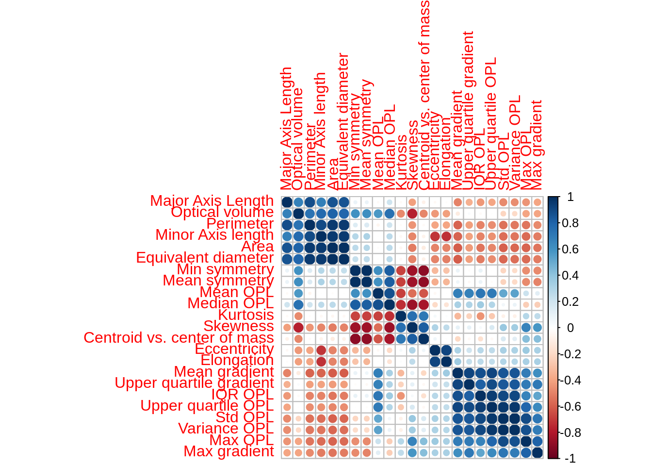
Find highly correlated predictors
## [1] 15## [1] "Max OPL" "Std OPL"
## [3] "Area" "Minor Axis length"
## [5] "Mean gradient" "Equivalent diameter"
## [7] "Variance OPL" "Skewness"
## [9] "IQR OPL" "Upper quartile gradient"
## [11] "Median OPL" "Mean symmetry"
## [13] "Min symmetry" "Major Axis Length"
## [15] "Elongation"G.2.4 Skewness
Observations grouped by infection status:
featurePlot(x = morphologyTrain,
            y = infectionStatusTrain,
            plot = "density",
            ## Pass in options to xyplot() to
            ## make it prettier
            scales = list(x = list(relation="free"),
                          y = list(relation="free")),
            adjust = 1.5,
            pch = "|",
            layout = c(5, 5),
            auto.key = list(columns = 2))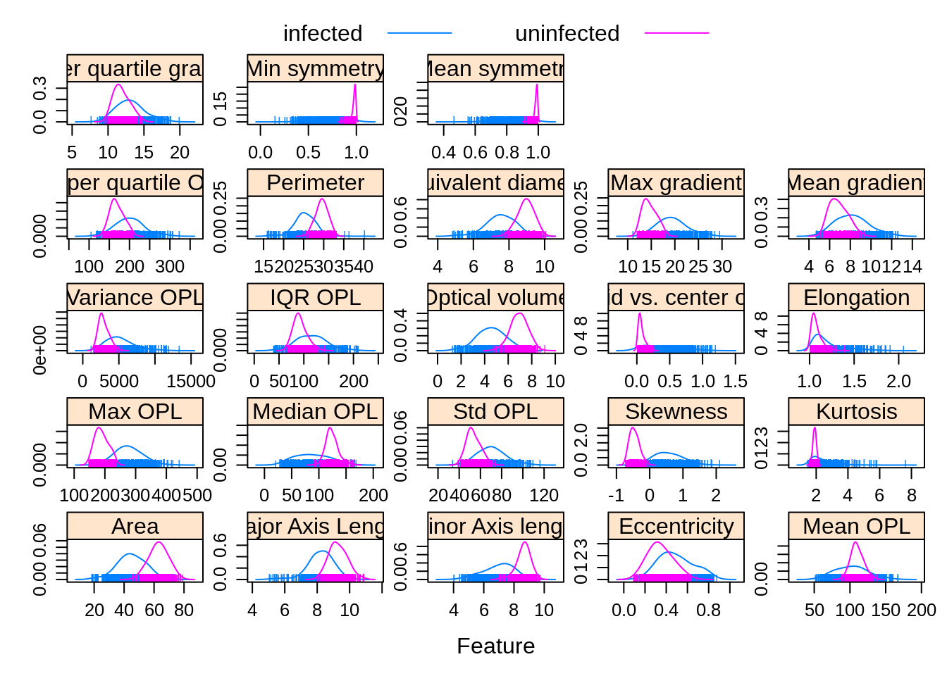
Observations grouped by infection stage:
featurePlot(x = morphologyTrain,
            y = stageTrain,
            plot = "density",
            ## Pass in options to xyplot() to
            ## make it prettier
            scales = list(x = list(relation="free"),
                          y = list(relation="free")),
            adjust = 1.5,
            pch = "|",
            layout = c(5, 5),
            auto.key = list(columns = 2))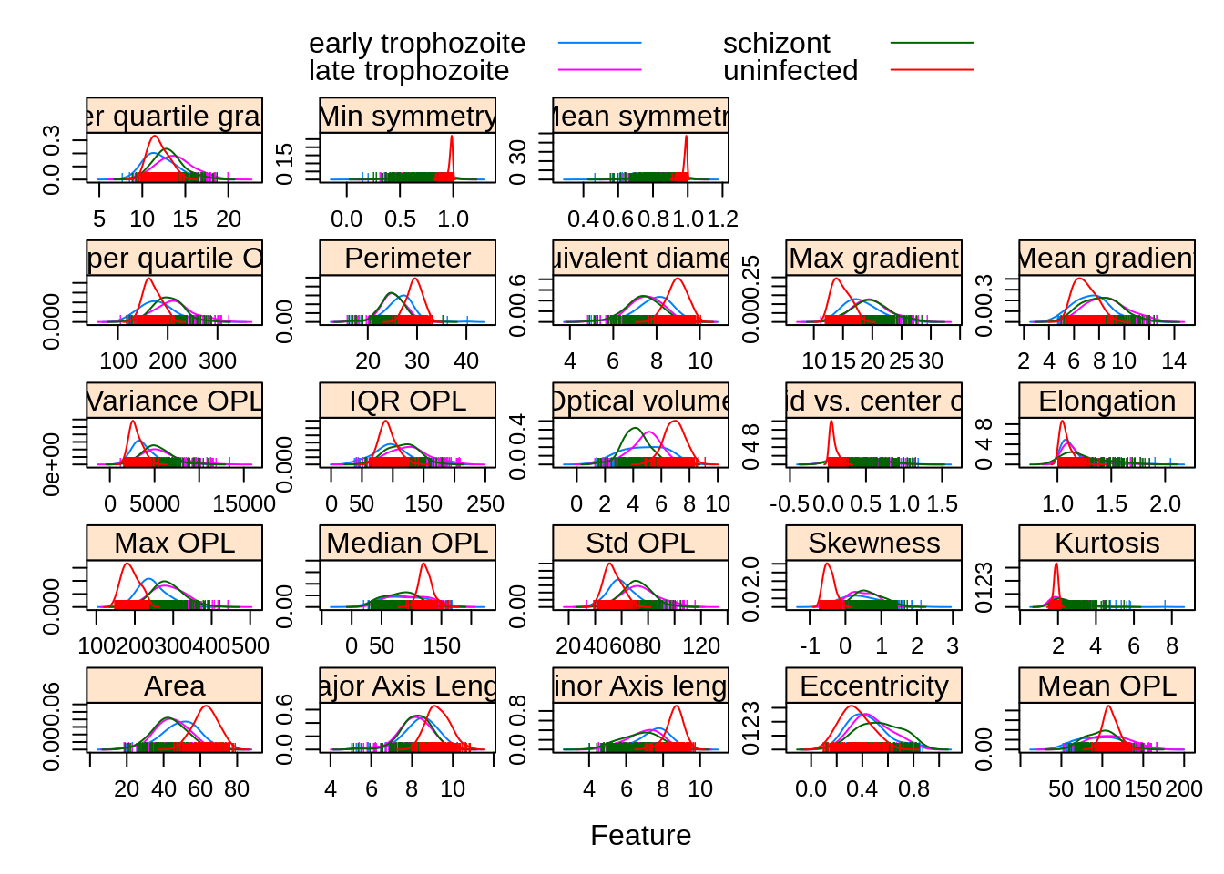
G.3 Infection status (two-class problem)
G.3.1 Model training and parameter tuning
All of the models we are going to use have a single tuning parameter. For each model we will use repeated cross validation to try 10 different values of the tuning parameter.
For each model let’s do five-fold cross-validation a total of five times. To make the analysis reproducible we need to specify the seed for each resampling iteration.
G.3.2 KNN
Train knn model:
knnFit <- train(morphologyTrain, infectionStatusTrain,
                method="knn",
                preProcess = c("center", "scale"),
                #tuneGrid=tuneParam,
                tuneLength=10,
                trControl=train_ctrl_infect_status)
## Warning in train.default(morphologyTrain, infectionStatusTrain, method =
## "knn", : The metric "Accuracy" was not in the result set. ROC will be used
## instead.## k-Nearest Neighbors
##
## 868 samples
## 23 predictor
## 2 classes: 'infected', 'uninfected'
##
## Pre-processing: centered (23), scaled (23)
## Resampling: Cross-Validated (5 fold, repeated 5 times)
## Summary of sample sizes: 695, 694, 695, 694, 694, 695, ...
## Resampling results across tuning parameters:
##
## k ROC Sens Spec
## 5 0.9962939 0.9716012 0.9979310
## 7 0.9963053 0.9688396 0.9986207
## 9 0.9959917 0.9653793 0.9965517
## 11 0.9958366 0.9646897 0.9951724
## 13 0.9958165 0.9646957 0.9965517
## 15 0.9961136 0.9640030 0.9958621
## 17 0.9963648 0.9640060 0.9944828
## 19 0.9961856 0.9619280 0.9958621
## 21 0.9960810 0.9615832 0.9944828
## 23 0.9959707 0.9608966 0.9951724
##
## ROC was used to select the optimal model using the largest value.
## The final value used for the model was k = 17.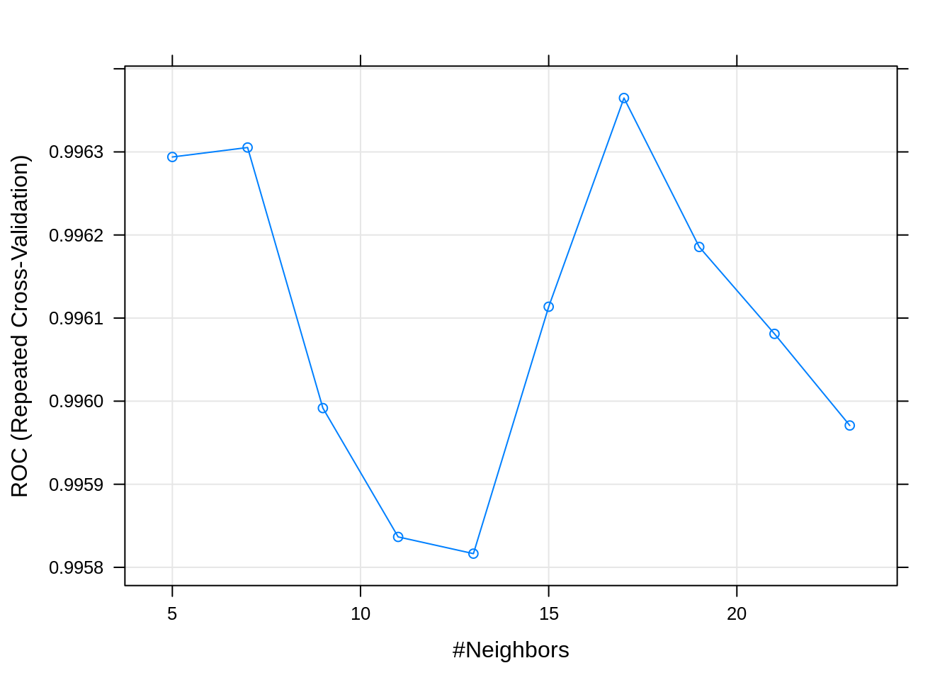
G.3.3 SVM
Train svm model:
svmFit <- train(morphologyTrain, infectionStatusTrain,
                method=svmRadialE1071,
                preProcess = c("center", "scale"),
                #tuneGrid=tuneParam,
                tuneLength=10,
                trControl=train_ctrl_infect_status)
## Warning in train.default(morphologyTrain, infectionStatusTrain, method =
## svmRadialE1071, : The metric "Accuracy" was not in the result set. ROC will be
## used instead.## Support Vector Machines with Radial Kernel - e1071
##
## 868 samples
## 23 predictor
## 2 classes: 'infected', 'uninfected'
##
## Pre-processing: centered (23), scaled (23)
## Resampling: Cross-Validated (5 fold, repeated 5 times)
## Summary of sample sizes: 694, 694, 695, 694, 695, 695, ...
## Resampling results across tuning parameters:
##
## cost ROC Sens Spec
## 0.25 0.9973153 0.9733673 0.9917241
## 0.50 0.9975655 0.9737121 0.9972414
## 1.00 0.9977089 0.9754393 0.9993103
## 2.00 0.9979474 0.9785607 0.9993103
## 4.00 0.9978997 0.9813253 0.9972414
## 8.00 0.9978157 0.9833943 0.9972414
## 16.00 0.9975119 0.9858111 0.9965517
## 32.00 0.9975000 0.9875412 0.9958621
## 64.00 0.9973454 0.9892714 0.9944828
## 128.00 0.9964930 0.9892684 0.9910345
##
## ROC was used to select the optimal model using the largest value.
## The final value used for the model was cost = 2.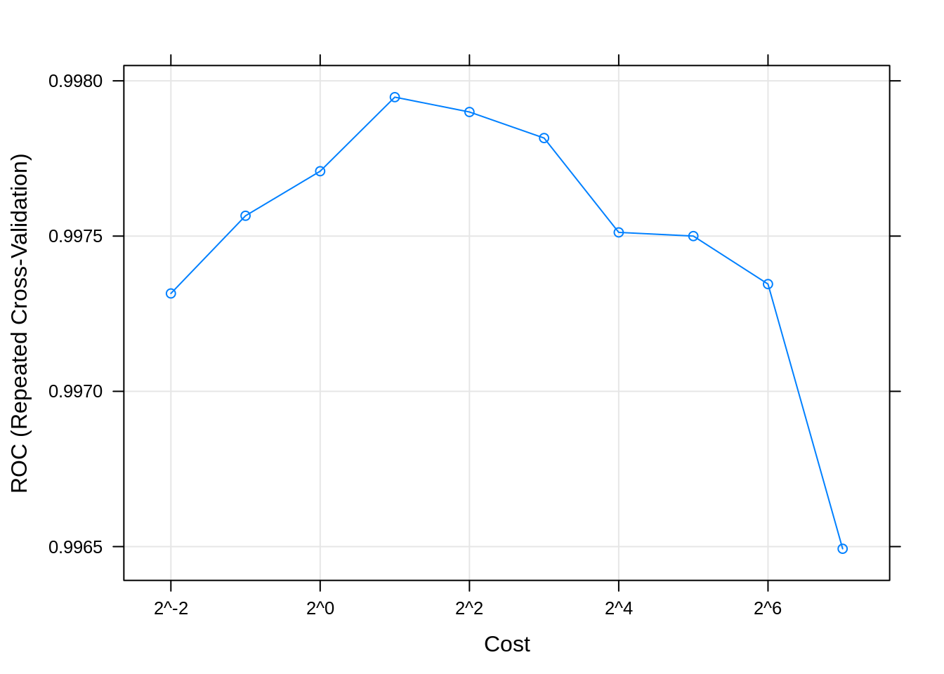
G.3.4 Decision tree
Train decision tree model:
dtFit <- train(morphologyTrain, infectionStatusTrain,
                method="rpart",
                preProcess = c("center", "scale"),
                #tuneGrid=tuneParam,
                tuneLength=10,
                trControl=train_ctrl_infect_status)
## Warning in train.default(morphologyTrain, infectionStatusTrain, method =
## "rpart", : The metric "Accuracy" was not in the result set. ROC will be used
## instead.## CART
##
## 868 samples
## 23 predictor
## 2 classes: 'infected', 'uninfected'
##
## Pre-processing: centered (23), scaled (23)
## Resampling: Cross-Validated (5 fold, repeated 5 times)
## Summary of sample sizes: 694, 694, 694, 695, 695, 694, ...
## Resampling results across tuning parameters:
##
## cp ROC Sens Spec
## 0.0000000 0.9824943 0.9771634 0.9779310
## 0.1003831 0.9652759 0.9574483 0.9731034
## 0.2007663 0.9652759 0.9574483 0.9731034
## 0.3011494 0.9652759 0.9574483 0.9731034
## 0.4015326 0.9652759 0.9574483 0.9731034
## 0.5019157 0.9652759 0.9574483 0.9731034
## 0.6022989 0.9652759 0.9574483 0.9731034
## 0.7026820 0.9652759 0.9574483 0.9731034
## 0.8030651 0.9652759 0.9574483 0.9731034
## 0.9034483 0.7758156 0.9723208 0.5793103
##
## ROC was used to select the optimal model using the largest value.
## The final value used for the model was cp = 0.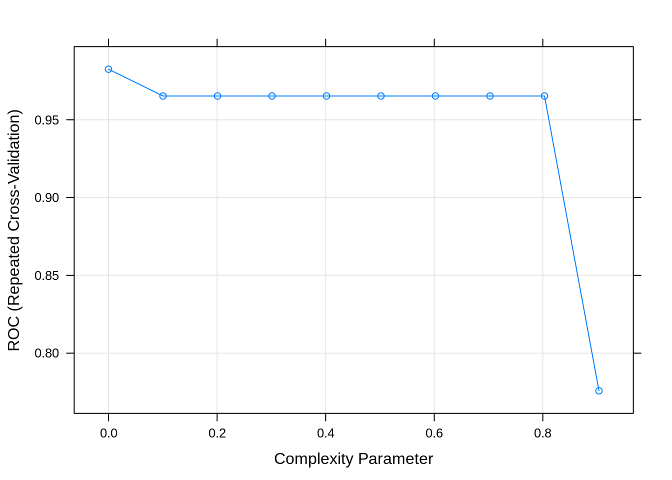

G.3.5 Random forest
rfFit <- train(morphologyTrain, infectionStatusTrain,
                method="rf",
                preProcess = c("center", "scale"),
                #tuneGrid=tuneParam,
                tuneLength=10,
                trControl=train_ctrl_infect_status)
## Warning in train.default(morphologyTrain, infectionStatusTrain, method = "rf", :
## The metric "Accuracy" was not in the result set. ROC will be used instead.## Random Forest
##
## 868 samples
## 23 predictor
## 2 classes: 'infected', 'uninfected'
##
## Pre-processing: centered (23), scaled (23)
## Resampling: Cross-Validated (5 fold, repeated 5 times)
## Summary of sample sizes: 694, 694, 695, 694, 695, 695, ...
## Resampling results across tuning parameters:
##
## mtry ROC Sens Spec
## 2 0.9979473 0.9871994 0.9834483
## 4 0.9976783 0.9871994 0.9827586
## 6 0.9973155 0.9865067 0.9882759
## 9 0.9973173 0.9858141 0.9868966
## 11 0.9967869 0.9851154 0.9862069
## 13 0.9968942 0.9840780 0.9848276
## 16 0.9965961 0.9840750 0.9820690
## 18 0.9964142 0.9830435 0.9793103
## 20 0.9960719 0.9820030 0.9806897
## 23 0.9940873 0.9813133 0.9806897
##
## ROC was used to select the optimal model using the largest value.
## The final value used for the model was mtry = 2.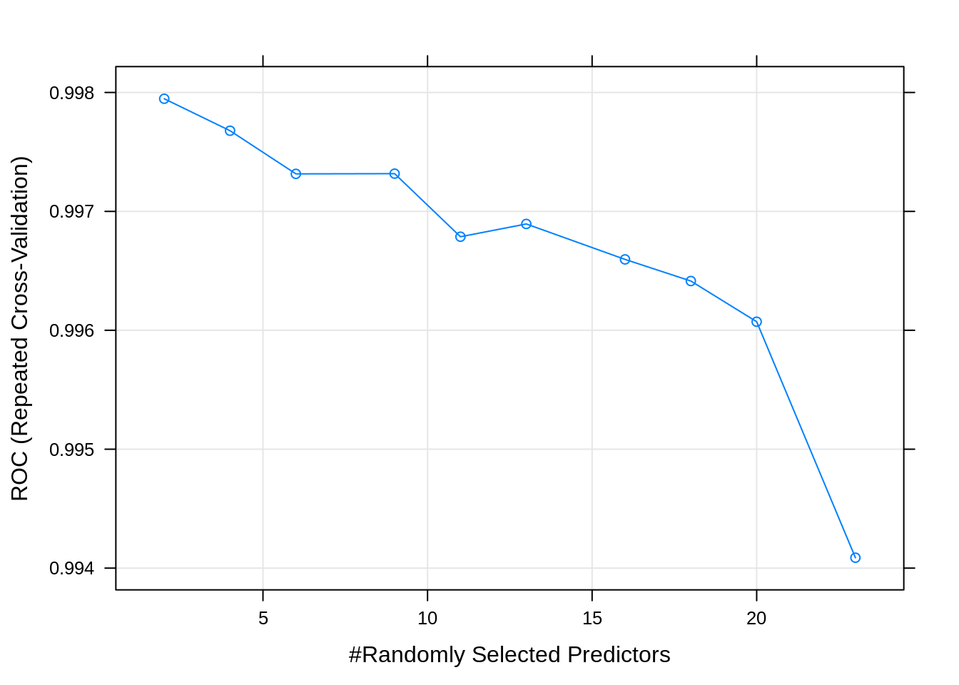
G.3.6 Compare models
Make a list of our models
Collect resampling results for each model
##
## Call:
## resamples.default(x = model_list)
##
## Models: knn, svm, decisionTree, randomForest
## Number of resamples: 25
## Performance metrics: ROC, Sens, Spec
## Time estimates for: everything, final model fit##
## Call:
## summary.resamples(object = resamps)
##
## Models: knn, svm, decisionTree, randomForest
## Number of resamples: 25
##
## ROC
## Min. 1st Qu. Median Mean 3rd Qu. Max. NA's
## knn 0.9865817 0.9940547 0.9979760 0.9963648 0.9991082 0.9999257 0
## svm 0.9937031 0.9965815 0.9994055 0.9979474 0.9997027 1.0000000 0
## decisionTree 0.9656659 0.9743609 0.9818668 0.9824943 0.9906297 0.9999257 0
## randomForest 0.9940780 0.9966558 0.9991082 0.9979473 0.9997001 1.0000000 0
##
## Sens
## Min. 1st Qu. Median Mean 3rd Qu. Max. NA's
## knn 0.9304348 0.9568966 0.9655172 0.9640060 0.9741379 0.9913043 0
## svm 0.9396552 0.9739130 0.9827586 0.9785607 0.9913043 1.0000000 0
## decisionTree 0.9391304 0.9655172 0.9741379 0.9771634 0.9827586 1.0000000 0
## randomForest 0.9565217 0.9827586 0.9913043 0.9871994 0.9913793 1.0000000 0
##
## Spec
## Min. 1st Qu. Median Mean 3rd Qu. Max. NA's
## knn 0.9655172 0.9827586 1.0000000 0.9944828 1 1 0
## svm 0.9827586 1.0000000 1.0000000 0.9993103 1 1 0
## decisionTree 0.9482759 0.9655172 0.9827586 0.9779310 1 1 0
## randomForest 0.9310345 0.9655172 0.9827586 0.9834483 1 1 0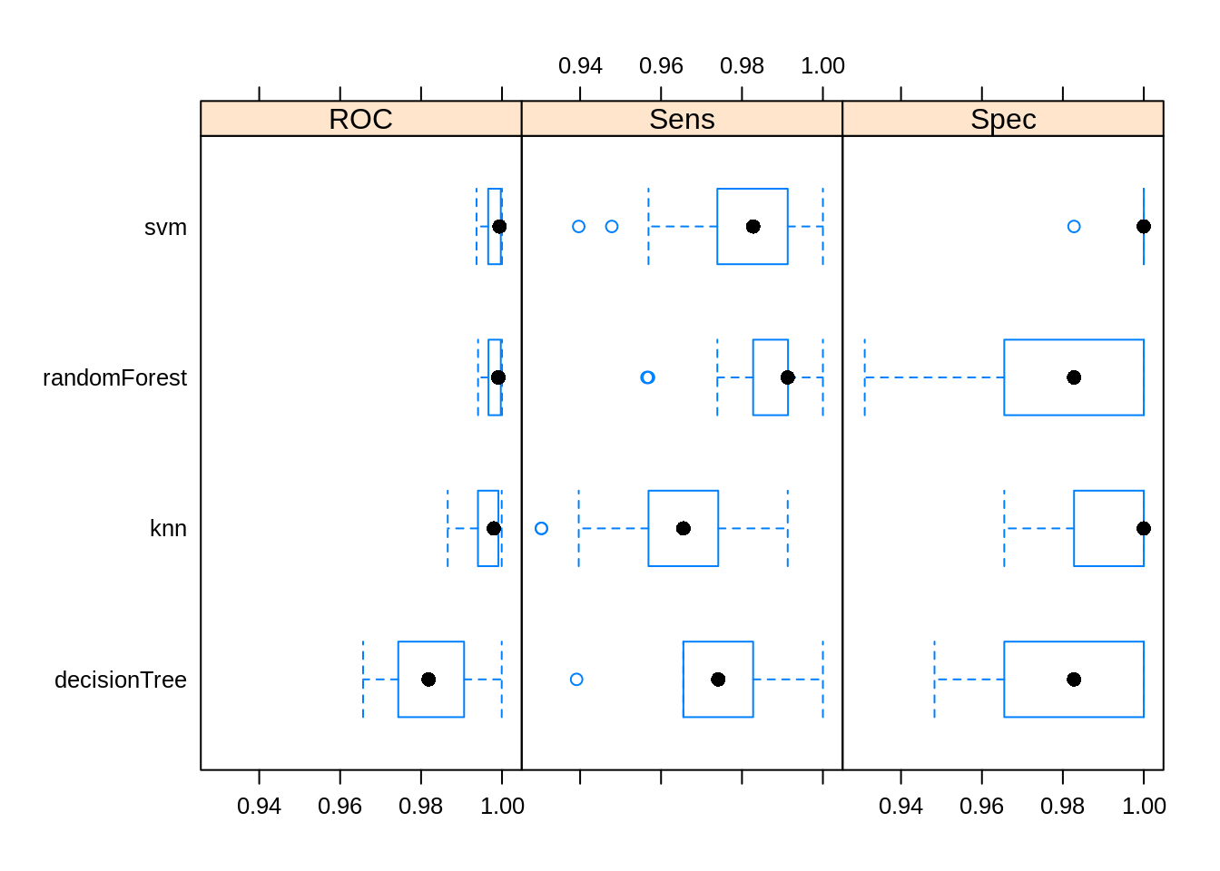
G.3.7 Predict test set using our best model
## Confusion Matrix and Statistics
##
##             Reference
## Prediction   infected uninfected
##   infected        246          2
##   uninfected        0        121
##
##                Accuracy : 0.9946
##                  95% CI : (0.9806, 0.9993)
##     No Information Rate : 0.6667
##     P-Value [Acc > NIR] : <2e-16
##
##                   Kappa : 0.9878
##
##  Mcnemar's Test P-Value : 0.4795
##
##             Sensitivity : 1.0000
##             Specificity : 0.9837
##          Pos Pred Value : 0.9919
##          Neg Pred Value : 1.0000
##              Prevalence : 0.6667
##          Detection Rate : 0.6667
##    Detection Prevalence : 0.6721
##       Balanced Accuracy : 0.9919
##
##        'Positive' Class : infected
##
G.3.8 ROC curve
##               infected uninfected
## normal_..7 0.585266476  0.4147335
## normal_.15 0.009865544  0.9901345
## normal_.23 0.004011000  0.9959890
## normal_.26 0.003558421  0.9964416
## normal_.29 0.049331293  0.9506687
## normal_.31 0.003040713 0.9969593## Setting levels: control = infected, case = uninfected## Setting direction: controls > cases## Area under the curve: 0.9998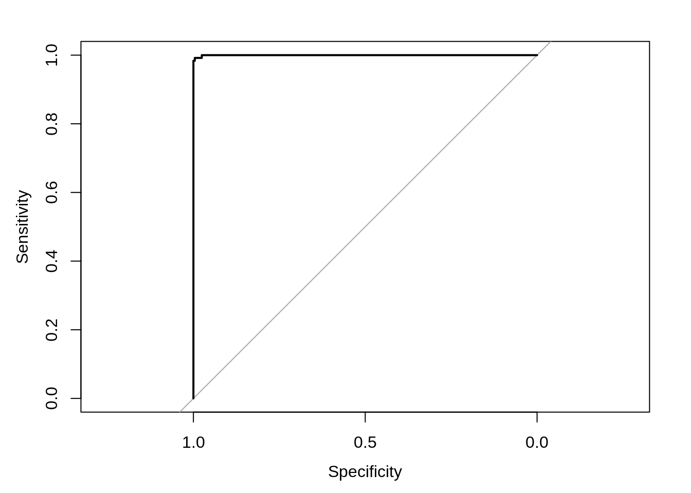
G.4 Discrimination of infective stages (multi-class problem)
G.4.1 Define cross-validation procedure
G.4.2 KNN
Train knn model with all variables:
knnFit <- train(morphologyTrain, stageTrain,
                method="knn",
                preProcess = c("center", "scale"),
                #tuneGrid=tuneParam,
                tuneLength=10,
                trControl=train_ctrl_stage)

knnFit
## k-Nearest Neighbors
##
## 868 samples
## 23 predictor
## 4 classes: 'early trophozoite', 'late trophozoite', 'schizont', 'uninfected'
##
## Pre-processing: centered (23), scaled (23)
## Resampling: Cross-Validated (5 fold, repeated 5 times)
## Summary of sample sizes: 695, 695, 694, 694, 694, 695, ...
## Resampling results across tuning parameters:
##
## k Accuracy Kappa
## 5 0.6868604 0.5665951
## 7 0.7009287 0.5851071
## 9 0.6990776 0.5817008
## 11 0.6990723 0.5810318
## 13 0.6967668 0.5777231
## 15 0.6956239 0.5757095
## 17 0.6939883 0.5731538
## 19 0.6951456 0.5746427
## 21 0.6935272 0.5723110
## 23 0.6863847 0.5621102
##
## Accuracy was used to select the optimal model using the largest value.
## The final value used for the model was k = 7.
G.4.3 SVM
Train SVM model with all variables:
svmFit <- train(morphologyTrain, stageTrain,
                method=svmRadialE1071,
                preProcess = c("center", "scale"),
                #tuneGrid=tuneParam,
                tuneLength=10,
                trControl=train_ctrl_stage)

svmFit
## Support Vector Machines with Radial Kernel - e1071
##
## 868 samples
## 23 predictor
## 4 classes: 'early trophozoite', 'late trophozoite', 'schizont', 'uninfected'
##
## Pre-processing: centered (23), scaled (23)
## Resampling: Cross-Validated (5 fold, repeated 5 times)
## Summary of sample sizes: 695, 694, 694, 694, 695, 695, ...
## Resampling results across tuning parameters:
##
## cost Accuracy Kappa
## 0.25 0.6965183 0.5770470
## 0.50 0.7131020 0.6018203
## 1.00 0.7213926 0.6141816
## 2.00 0.7220875 0.6157211
## 4.00 0.7292154 0.6260607
## 8.00 0.7333785 0.6326331
## 16.00 0.7241711 0.6206293
## 32.00 0.7094464 0.6008159
## 64.00 0.6972345 0.5847166
## 128.00 0.6903300 0.5758449
##
## Accuracy was used to select the optimal model using the largest value.
## The final value used for the model was cost = 8.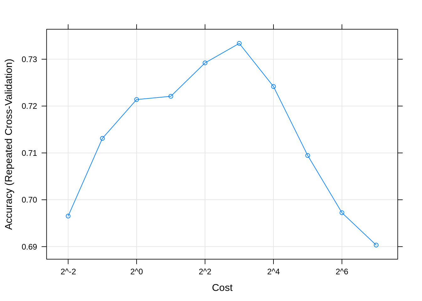
G.4.4 Decision tree
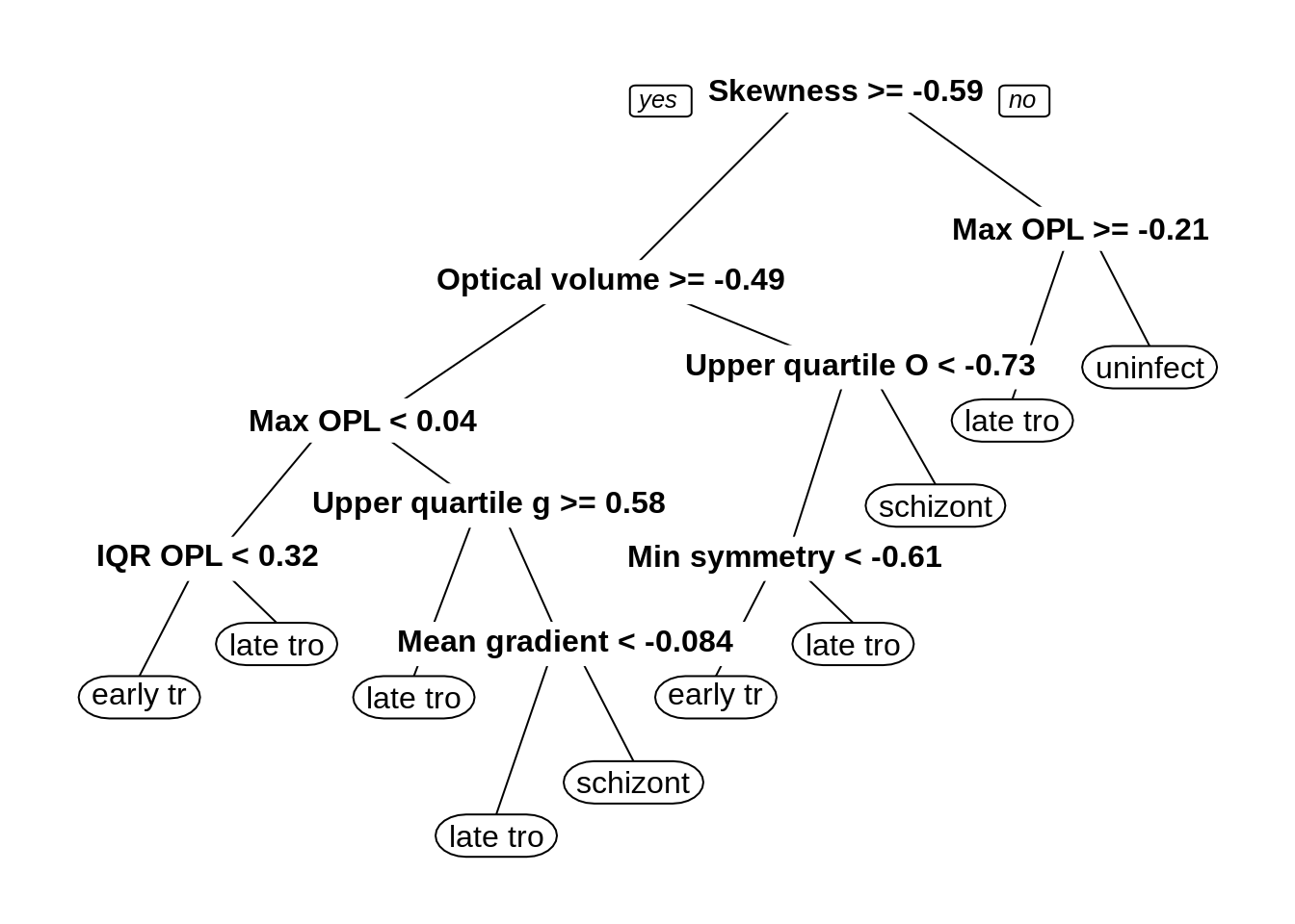
Train decision tree model with all variables:
dtFit <- train(morphologyTrain, stageTrain,
                method="rpart",
                preProcess = c("center", "scale"),
                #tuneGrid=tuneParam,
                tuneLength=10,
                trControl=train_ctrl_stage)

dtFit
## CART
##
## 868 samples
## 23 predictor
## 4 classes: 'early trophozoite', 'late trophozoite', 'schizont', 'uninfected'
##
## Pre-processing: centered (23), scaled (23)
## Resampling: Cross-Validated (5 fold, repeated 5 times)
## Summary of sample sizes: 695, 694, 694, 694, 695, 695, ...
## Resampling results across tuning parameters:
##
## cp Accuracy Kappa
## 0.004498270 0.6882662 0.5716210
## 0.005190311 0.6905585 0.5747141
## 0.006920415 0.6988530 0.5860335
## 0.012110727 0.6960917 0.5831319
## 0.013840830 0.6972398 0.5845125
## 0.015570934 0.6949355 0.5809362
## 0.025951557 0.6898488 0.5724806
## 0.031141869 0.6820128 0.5595580
## 0.119377163 0.6145431 0.4549600
## 0.399653979 0.4920449 0.2576226
##
## Accuracy was used to select the optimal model using the largest value.
## The final value used for the model was cp = 0.006920415.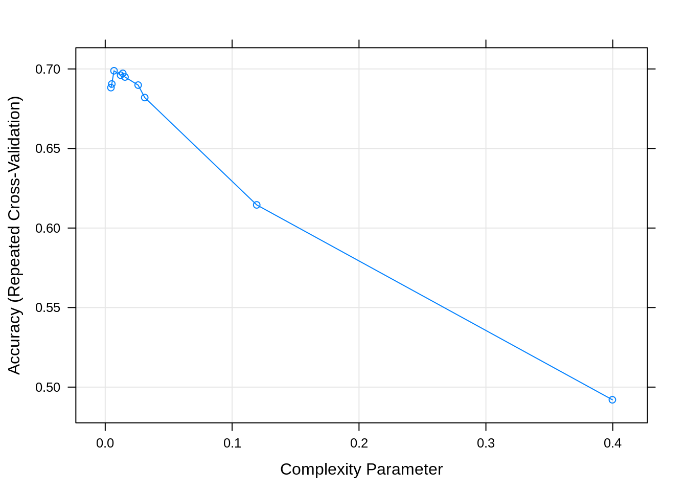
G.4.5 Random forest
Train random forest model with all variables:
rfFit <- train(morphologyTrain, stageTrain,
                method="rf",
                preProcess = c("center", "scale"),
                #tuneGrid=tuneParam,
                tuneLength=10,
                trControl=train_ctrl_stage)

rfFit
## Random Forest
##
## 868 samples
## 23 predictor
## 4 classes: 'early trophozoite', 'late trophozoite', 'schizont', 'uninfected'
##
## Pre-processing: centered (23), scaled (23)
## Resampling: Cross-Validated (5 fold, repeated 5 times)
## Summary of sample sizes: 695, 694, 694, 694, 695, 695, ...
## Resampling results across tuning parameters:
##
## mtry Accuracy Kappa
## 2 0.7228208 0.6176325
## 4 0.7221246 0.6173189
## 6 0.7274200 0.6246213
## 9 0.7219067 0.6171952
## 11 0.7202750 0.6149614
## 13 0.7170539 0.6105192
## 16 0.7209752 0.6161230
## 18 0.7235093 0.6196690
## 20 0.7230323 0.6190254
## 23 0.7232833 0.6195279
##
## Accuracy was used to select the optimal model using the largest value.
## The final value used for the model was mtry = 6.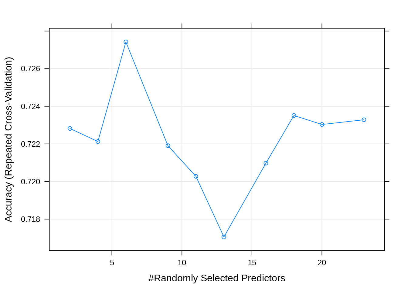
G.4.6 Compare models
Make a list of our models
Collect resampling results for each model
##
## Call:
## resamples.default(x = model_list)
##
## Models: knn, svm, decisionTree, randomForest
## Number of resamples: 25
## Performance metrics: Accuracy, Kappa
## Time estimates for: everything, final model fit##
## Call:
## summary.resamples(object = resamps)
##
## Models: knn, svm, decisionTree, randomForest
## Number of resamples: 25
##
## Accuracy
## Min. 1st Qu. Median Mean 3rd Qu. Max. NA's
## knn 0.6494253 0.6896552 0.6994220 0.7009287 0.7109827 0.7456647 0
## svm 0.6705202 0.7241379 0.7341040 0.7333785 0.7456647 0.7873563 0
## decisionTree 0.6473988 0.6705202 0.7011494 0.6988530 0.7225434 0.7572254 0
## randomForest 0.6763006 0.7011494 0.7298851 0.7274200 0.7514451 0.7919075 0
##
## Kappa
## Min. 1st Qu. Median Mean 3rd Qu. Max. NA's
## knn 0.5123139 0.5676422 0.5827265 0.5851071 0.5998149 0.6473804 0
## svm 0.5440211 0.6195682 0.6331301 0.6326331 0.6489416 0.7081066 0
## decisionTree 0.5120226 0.5490818 0.5853726 0.5860335 0.6163371 0.6688995 0
## randomForest 0.5542058 0.5873584 0.6284754 0.6246213 0.6584168 0.7119734 0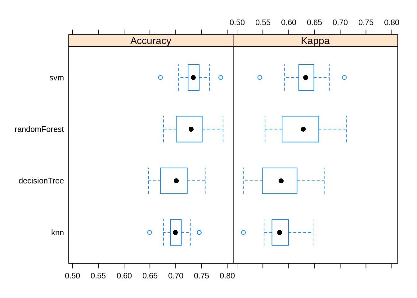
G.4.7 Predict test set using our best model
## Confusion Matrix and Statistics
##
##                    Reference
## Prediction          early trophozoite late trophozoite schizont uninfected
##   early trophozoite                27                9        6          3
##   late trophozoite                 10               54       29          1
##   schizont                         13               31       66          0
##   uninfected                        1                0        0        119
##
## Overall Statistics
##
##                Accuracy : 0.7209
##                  95% CI : (0.6721, 0.7661)
##     No Information Rate : 0.3333
##     P-Value [Acc > NIR] : < 2.2e-16
##
##                   Kappa : 0.6167
##
##  Mcnemar's Test P-Value : NA
##
## Statistics by Class:
##
##                      Class: early trophozoite Class: late trophozoite
## Sensitivity                           0.52941                  0.5745
## Specificity                           0.94340                  0.8545
## Pos Pred Value                        0.60000                  0.5745
## Neg Pred Value                        0.92593                  0.8545
## Prevalence                            0.13821                  0.2547
## Detection Rate                        0.07317                  0.1463
## Detection Prevalence                  0.12195                  0.2547
## Balanced Accuracy                     0.73640                  0.7145
##                      Class: schizont Class: uninfected
## Sensitivity                   0.6535            0.9675
## Specificity                   0.8358            0.9959
## Pos Pred Value                0.6000            0.9917
## Neg Pred Value                0.8649            0.9839
## Prevalence                    0.2737            0.3333
## Detection Rate                0.1789            0.3225
## Detection Prevalence          0.2981            0.3252
## Balanced Accuracy             0.7446            0.9817