6 Support vector machines
6.1 Introduction
Support vector machines (SVMs) are models of supervised learning, applicable to both classification and regression problems. The SVM is an extension of the support vector classifier (SVC), which is turn is an extension of the maximum margin classifier.
6.1.1 Maximum margin classifier
Let’s start by definining a hyperplane. In p-dimensional space a hyperplane is a flat affine subspace of p-1. Figure 6.1 shows three separating hyperplanes and objects of two different classes. A separating hyperplane forms a natural linear decision boundary, classifying new objects according to which side of the line they are located.
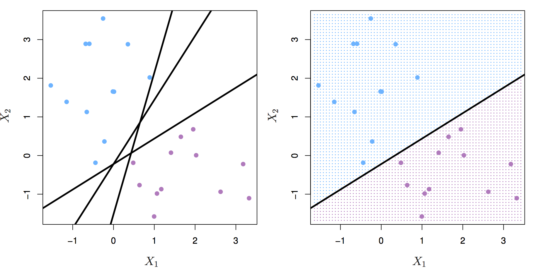
Figure 6.1: Left: two classes of observations (blue, purple) and three separating hyperplanes. Right: separating hyperplane shown as black line and grid indicates decision rule. Source: http://www-bcf.usc.edu/~gareth/ISL/
If the classes of observations can be separated by a hyperplane, then there will in fact be an infinite number of hyperplanes. So which of the possible hyperplanes do we choose to be our decision boundary?
The maximal margin hyperplane is the separating hyperplane that is farthest from the training observations. The perpendicular distance from a given hyperplane to the nearest training observation is known as the margin. The maximal margin hyperplane is the separating hyperplane for which the margin is largest.
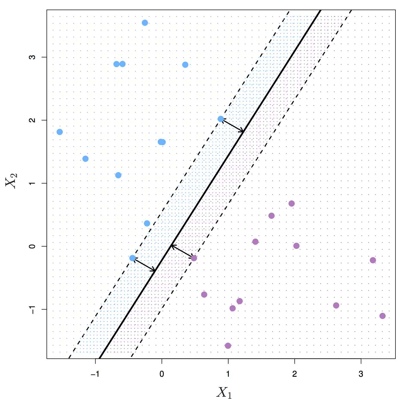
Figure 6.2: Maximal margin hyperplane shown as solid line. Margin is the distance from the solid line to either of the dashed lines. The support vectors are the points on the dashed line. Source: http://www-bcf.usc.edu/~gareth/ISL/
Figure 6.2 shows three training observations that are equidistant from the maximal margin hyperplane and lie on the dashed lines indicating the margin. These are the support vectors. If these points were moved slightly, the maximal margin hyperplane would also move, hence the term support. The maximal margin hyperplane is set by the support vectors alone; it is not influenced by any other observations.
The maximal margin hyperplane is a natural decision boundary, but only if a separating hyperplane exists. In practice there may be non separable cases which prevent the use of the maximal margin classifier.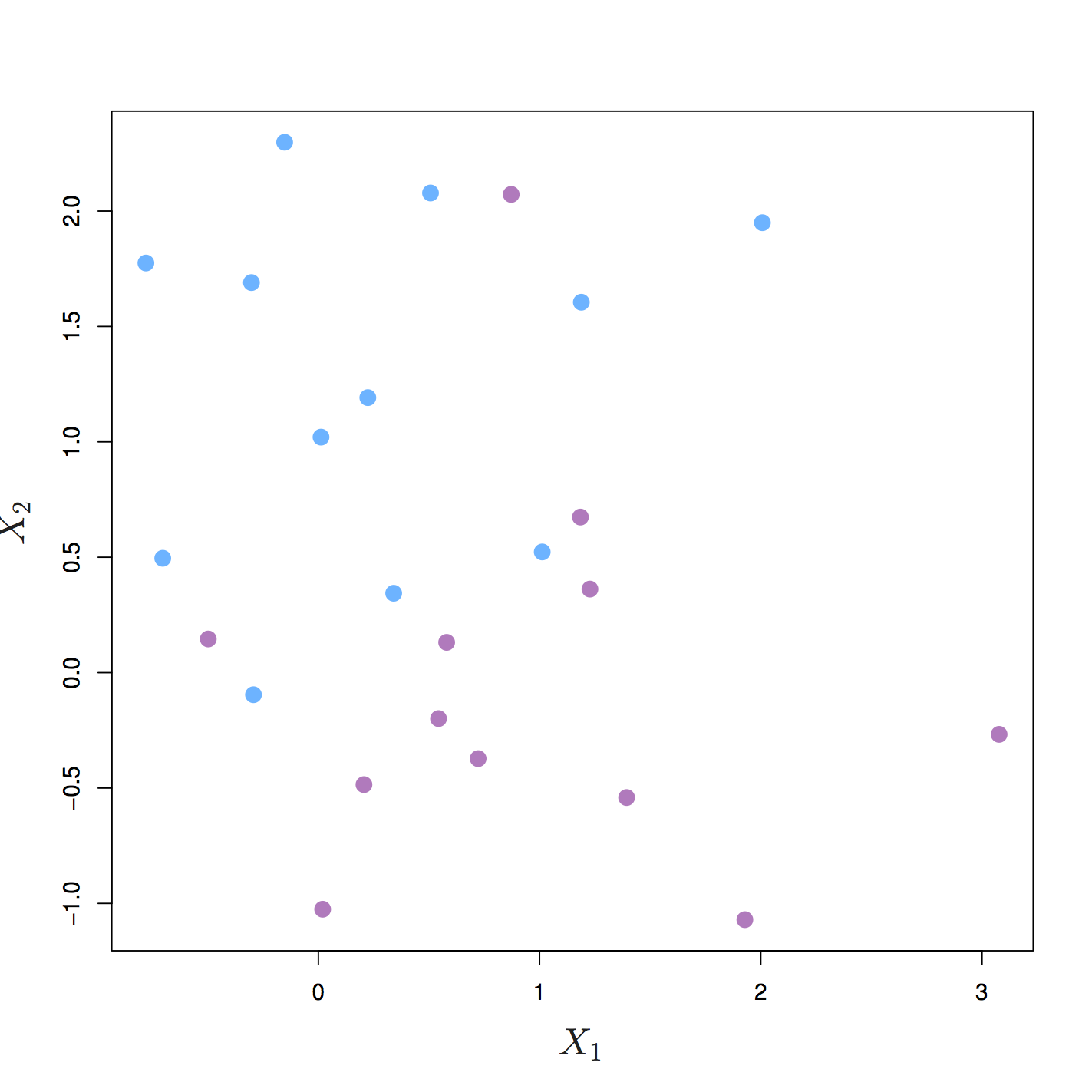
Figure 6.3: The two classes cannot be separated by a hyperplane and so the maximal margin classifier cannot be used. Source: http://www-bcf.usc.edu/~gareth/ISL/
6.2 Support vector classifier
Even if a separating hyperplane exists, it may not be the best decision boundary. The maximal margin classifier is extremely sensitive to individual observations, so may overfit the training data.
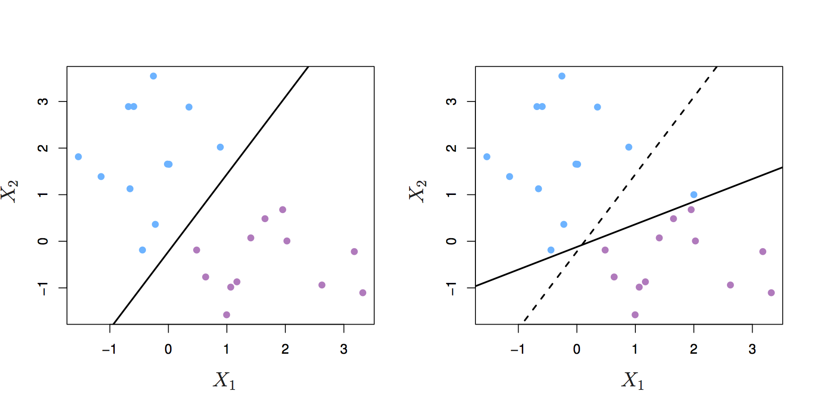
Figure 6.4: Left: two classes of observations and a maximum margin hyperplane (solid line). Right: Hyperplane (solid line) moves after the addition of a new observation (original hyperplane is dashed line). Source: http://www-bcf.usc.edu/~gareth/ISL/
It would be better to choose a classifier based on a hyperplane that:
- is more robust to individual observations
- provides better classification of most of the training variables
In other words, we might tolerate some misclassifications if the prediction of the remaining observations is more reliable. The support vector classifier does this by allowing some observations to be on the wrong side of the margin or even on the wrong side of the hyperplane. Observations on the wrong side of the hyperplane are misclassifications.
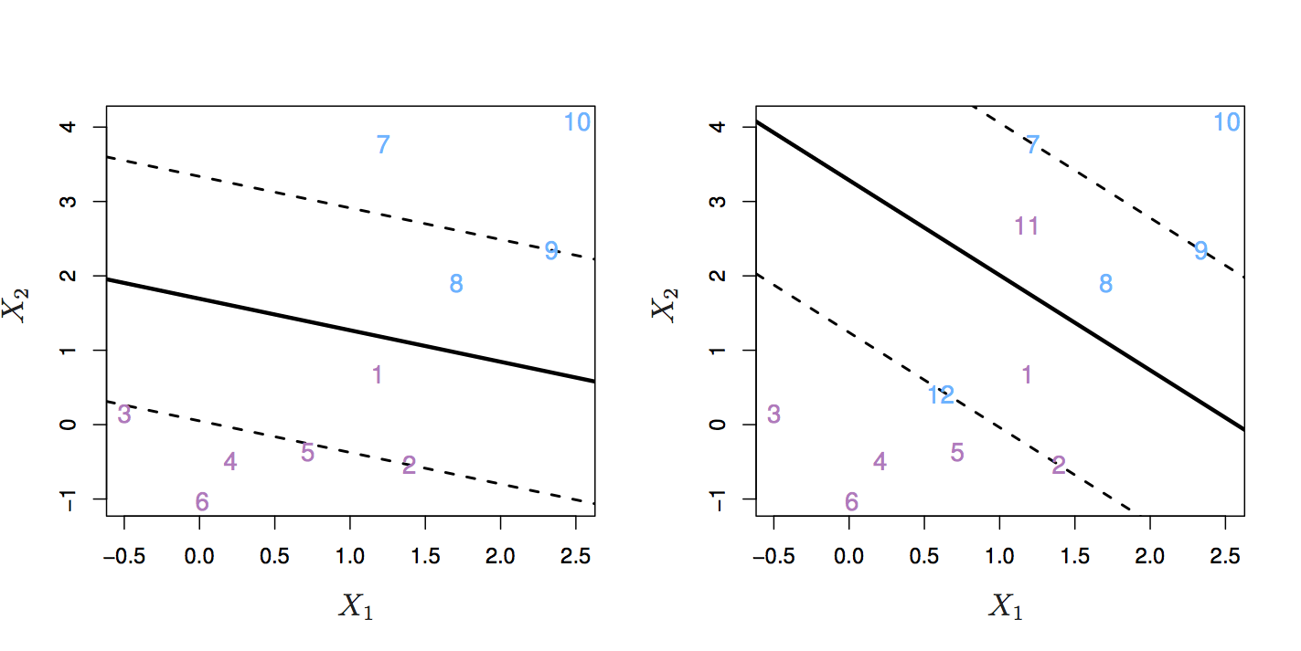
Figure 6.5: Left: observations on the wrong side of the margin. Right: observations on the wrong side of the margin and observations on the wrong side of the hyperplane. Source: http://www-bcf.usc.edu/~gareth/ISL/
The support vector classifier has a tuning parameter, C, that determines the number and severity of the violations to the margin. If C = 0, then no violations to the margin will be tolerated, which is equivalent to the maximal margin classifier. As C increases, the classifier becomes more tolerant of violations to the margin, and so the margin widens.
The optimal value of C is chosen through cross-validation.
C is described as a tuning parameter, because it controls the bias-variance trade-off:
- a small C results in narrow margins that are rarely violated; the model will have low bias, but high variance.
- as C increases the margins widen allowing more violations; the bias of the model will increase, but its variance will decrease.
The support vectors are the observations that lie directly on the margin, or on the wrong side of the margin for their class. The only observations that affect the classifier are the support vectors. As C increases, the margin widens and the number of support vectors increases. In other words, when C increases more observations are involved in determining the decision boundary of the classifier.
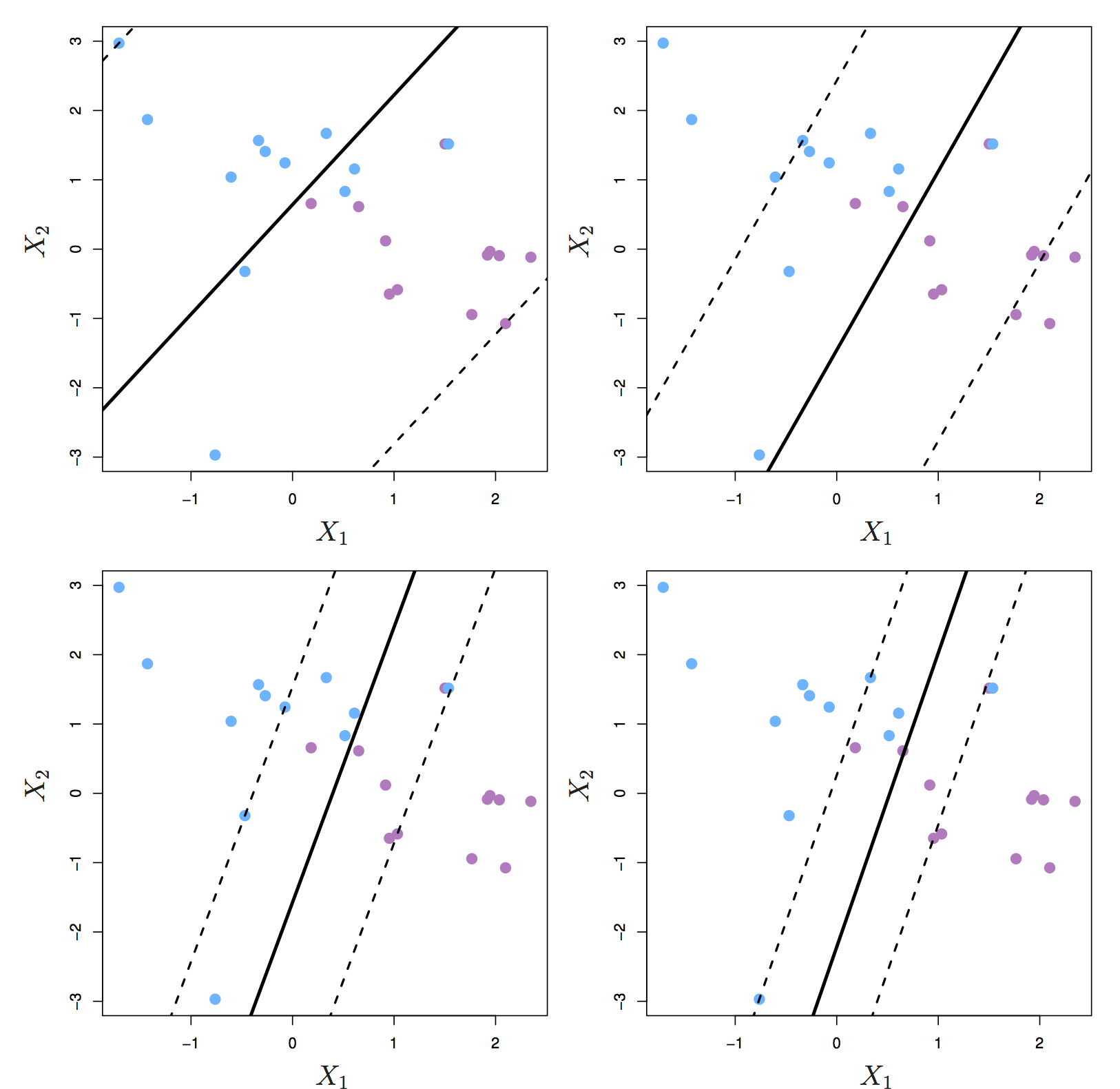
Figure 6.6: Margin of a support vector classifier changing with tuning parameter C. Largest value of C was used in the top left panel, and smaller values in the top right, bottom left and bottom right panels. Source: http://www-bcf.usc.edu/~gareth/ISL/
6.3 Support Vector Machine
The support vector classifier performs well if we have linearly separable classes, however this isn’t always the case.
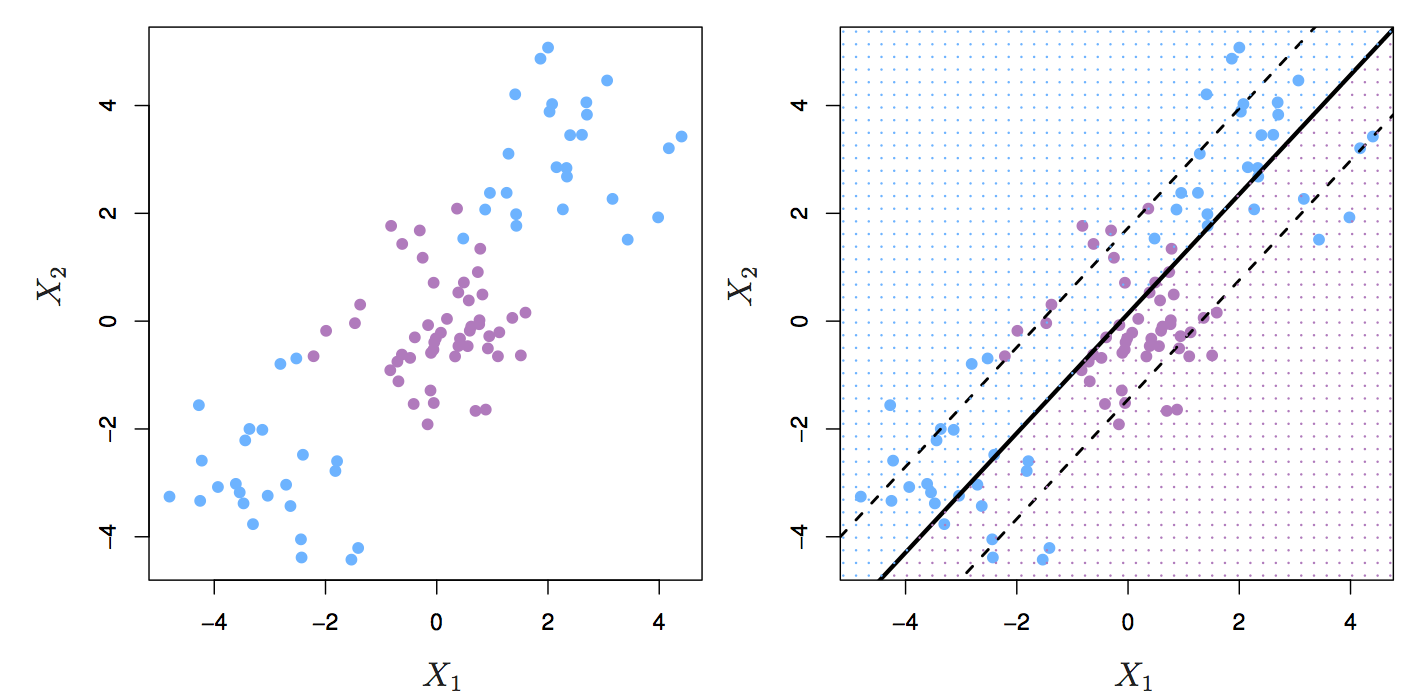
Figure 6.7: Two classes of observations with a non-linear boundary between them.
The SVM uses the kernel trick to operate in a higher dimensional space, without ever computing the coordinates of the data in that space.
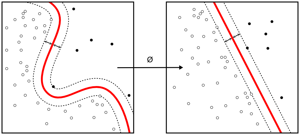
Figure 6.8: Kernel machine. By Alisneaky - Own work, CC0, https://commons.wikimedia.org/w/index.php?curid=14941564
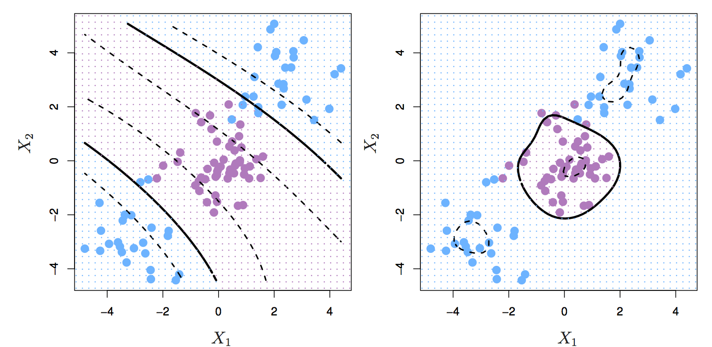
Figure 6.9: Left: SVM with polynomial kernel of degree 3. Right: SVM with radial kernel. Source: http://www-bcf.usc.edu/~gareth/ISL/
6.4 Example - training a classifier
Training of an SVM will be demonstrated on a 2-dimensional simulated data set, with a non-linear decision boundary.
6.4.1 Setup environment
Load required libraries
library(caret)## Warning in system("timedatectl", intern = TRUE): running command 'timedatectl'
## had status 1library(RColorBrewer)
library(ggplot2)
library(pROC)
library(e1071)6.4.2 Partition data
Load data
moons <- read.csv("data/sim_data_svm/moons.csv", header=F)
moons$V3=as.factor(moons$V3)
str(moons)
## 'data.frame': 400 obs. of 3 variables:
## $ V1: num -0.496 1.827 1.322 -1.138 -0.21 ...
## $ V2: num 0.985 -0.501 -0.397 0.192 -0.145 ...
## $ V3: Factor w/ 2 levels "A","B": 1 2 2 1 2 1 1 2 1 2 ...V1 and V2 are the predictors; V3 is the class.
Partition data into training and test set
set.seed(42)
trainIndex <- createDataPartition(y=moons$V3, times=1, p=0.7, list=F)
moonsTrain <- moons[trainIndex,]
moonsTest <- moons[-trainIndex,]

summary(moonsTrain$V3)
## A B
## 140 140summary(moonsTest$V3)## A B
## 60 606.4.3 Visualize training data
point_shapes <- c(15,17)
bp <- brewer.pal(3,"Dark2")
point_colours <- ifelse(moonsTrain$V3=="A", bp[1], bp[2])
point_shapes <- ifelse(moonsTrain$V3=="A", 15, 17)

point_size = 2

ggplot(moonsTrain, aes(V1,V2)) +
  geom_point(col=point_colours, shape=point_shapes,
             size=point_size) +
  theme_bw() +
  theme(plot.title = element_text(size=25, face="bold"), axis.text=element_text(size=15),
        axis.title=element_text(size=20,face="bold"))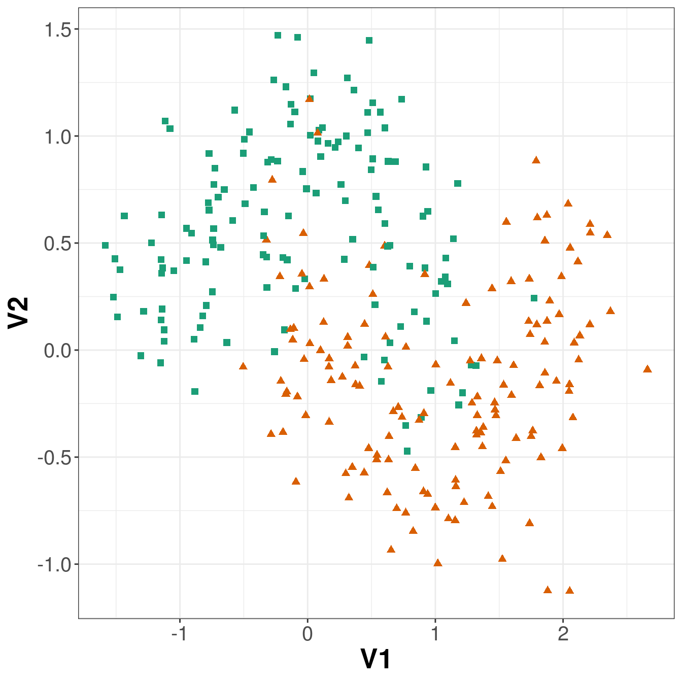
Figure 6.10: Scatterplot of the training data
set.seed(42)
seeds = vector(mode='list',length=101) #this is #folds+1 so 10+1
for (i in 1:100) seeds[[i]] = sample.int(1000,100)
seeds[[101]] = sample.int(1000,1)

trctrl <- trainControl(method = "repeatedcv",
                       number = 10,
                       repeats = 10,
                       seeds = seeds,
                       classProbs=TRUE)
svmTune <- train(x = moonsTrain[,c(1:2)],
                 y = moonsTrain[,3],
                 method = "svmRadial",
                 tuneLength = 9,
                 preProc = c("center", "scale"),
                 trControl = trctrl)

svmTune
## Support Vector Machines with Radial Basis Function Kernel
##
## 280 samples
## 2 predictor
## 2 classes: 'A', 'B'
##
## Pre-processing: centered (2), scaled (2)
## Resampling: Cross-Validated (10 fold, repeated 10 times)
## Summary of sample sizes: 252, 252, 252, 252, 252, 252, ...
## Resampling results across tuning parameters:
##
## C Accuracy Kappa
## 0.25 0.8875000 0.7750000
## 0.50 0.8846429 0.7692857
## 1.00 0.8810714 0.7621429
## 2.00 0.8803571 0.7607143
## 4.00 0.8750000 0.7500000
## 8.00 0.8671429 0.7342857
## 16.00 0.8635714 0.7271429
## 32.00 0.8582143 0.7164286
## 64.00 0.8557143 0.7114286
##
## Tuning parameter 'sigma' was held constant at a value of 1.36437
## Accuracy was used to select the optimal model using the largest value.
## The final values used for the model were sigma = 1.36437 and C = 0.25.6.4.4 Prediction performance measures
SVM accuracy profile
Predictions on test set.
svmPred <- predict(svmTune, moonsTest[,c(1:2)])
confusionMatrix(svmPred, as.factor(moonsTest[,3]))
## Confusion Matrix and Statistics
##
## Reference
## Prediction A B
## A 59 7
## B 1 53
##
## Accuracy : 0.9333
## 95% CI : (0.8729, 0.9708)
## No Information Rate : 0.5
## P-Value [Acc > NIR] : <2e-16
##
## Kappa : 0.8667
##
## Mcnemar's Test P-Value : 0.0771
##
## Sensitivity : 0.9833
## Specificity : 0.8833
## Pos Pred Value : 0.8939
## Neg Pred Value : 0.9815
## Prevalence : 0.5000
## Detection Rate : 0.4917
## Detection Prevalence : 0.5500
## Balanced Accuracy : 0.9333
##
## 'Positive' Class : A
## Get predicted class probabilities so we can build ROC curve.
svmProbs <- predict(svmTune, moonsTest[,c(1:2)], type="prob")
head(svmProbs)
## A B
## 1 0.06967502 0.93032498
## 2 0.93443571 0.06556429
## 3 0.93707422 0.06292578
## 4 0.07198768 0.92801232
## 5 0.88761226 0.11238774
## 6 0.94212490 0.05787510Build a ROC curve.
svmROC <- roc(moonsTest[,3], svmProbs[,"A"])## Setting levels: control = A, case = B## Setting direction: controls > casesPlot ROC curve.
plot(svmROC, type = "S")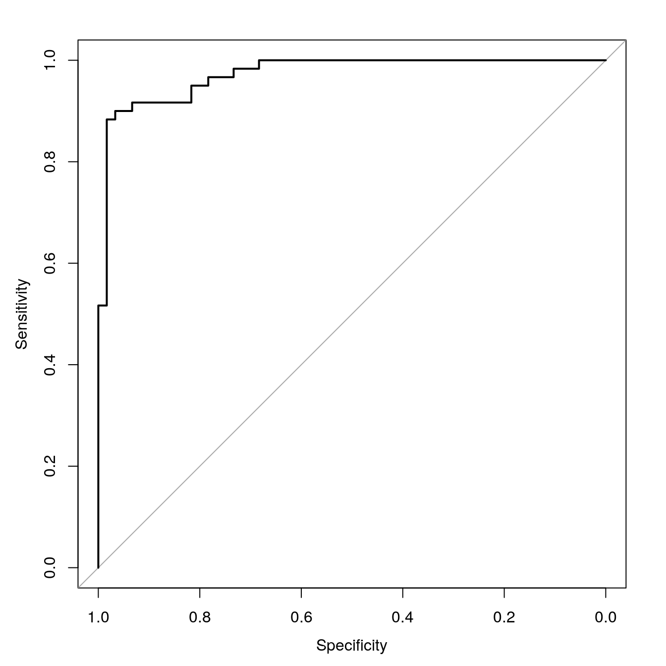
Figure 6.11: SVM accuracy profile.
Sensitivity (true positive rate)
TPR = TP/P = TP/(TP+FN)
Specificity (true negative rate)
SPC = TN/N = TN/(TN+FP)
Calculate area under ROC curve.
auc(svmROC)## Area under the curve: 0.97286.4.5 Plot decision boundary
Create a grid so we can predict across the full range of our variables V1 and V2.
gridSize <- 150
v1limits <- c(min(moons$V1),max(moons$V1))
tmpV1 <- seq(v1limits[1],v1limits[2],len=gridSize)
v2limits <- c(min(moons$V2), max(moons$V2))
tmpV2 <- seq(v2limits[1],v2limits[2],len=gridSize)
xgrid <- expand.grid(tmpV1,tmpV2)
names(xgrid) <- names(moons)[1:2]
Predict values of all elements of grid.
V3 <- as.numeric(predict(svmTune, xgrid))
xgrid <- cbind(xgrid, V3)
Plot
point_shapes <- c(15,17)
point_colours <- brewer.pal(3,"Dark2")
point_size = 2

trainClassNumeric <- ifelse(moonsTrain$V3=="A", 1, 2)
testClassNumeric <- ifelse(moonsTest$V3=="A", 1, 2)

ggplot(xgrid, aes(V1,V2)) +
  geom_point(col=point_colours[V3], shape=16, size=0.3) +
  geom_point(data=moonsTrain, aes(V1,V2), col=point_colours[trainClassNumeric],
             shape=point_shapes[trainClassNumeric], size=point_size) +
  geom_contour(data=xgrid, aes(x=V1, y=V2, z=V3), breaks=1.5, col="grey30") +
  ggtitle("train") +
  theme_bw() +
  theme(plot.title = element_text(size=25, face="bold"), axis.text=element_text(size=15),
        axis.title=element_text(size=20,face="bold"))

ggplot(xgrid, aes(V1,V2)) +
  geom_point(col=point_colours[V3], shape=16, size=0.3) +
  geom_point(data=moonsTest, aes(V1,V2), col=point_colours[testClassNumeric],
             shape=point_shapes[testClassNumeric], size=point_size) +
  geom_contour(data=xgrid, aes(x=V1, y=V2, z=V3), breaks=1.5, col="grey30") +
  ggtitle("test") +
  theme_bw() +
  theme(plot.title = element_text(size=25, face="bold"), axis.text=element_text(size=15),
        axis.title=element_text(size=20,face="bold"))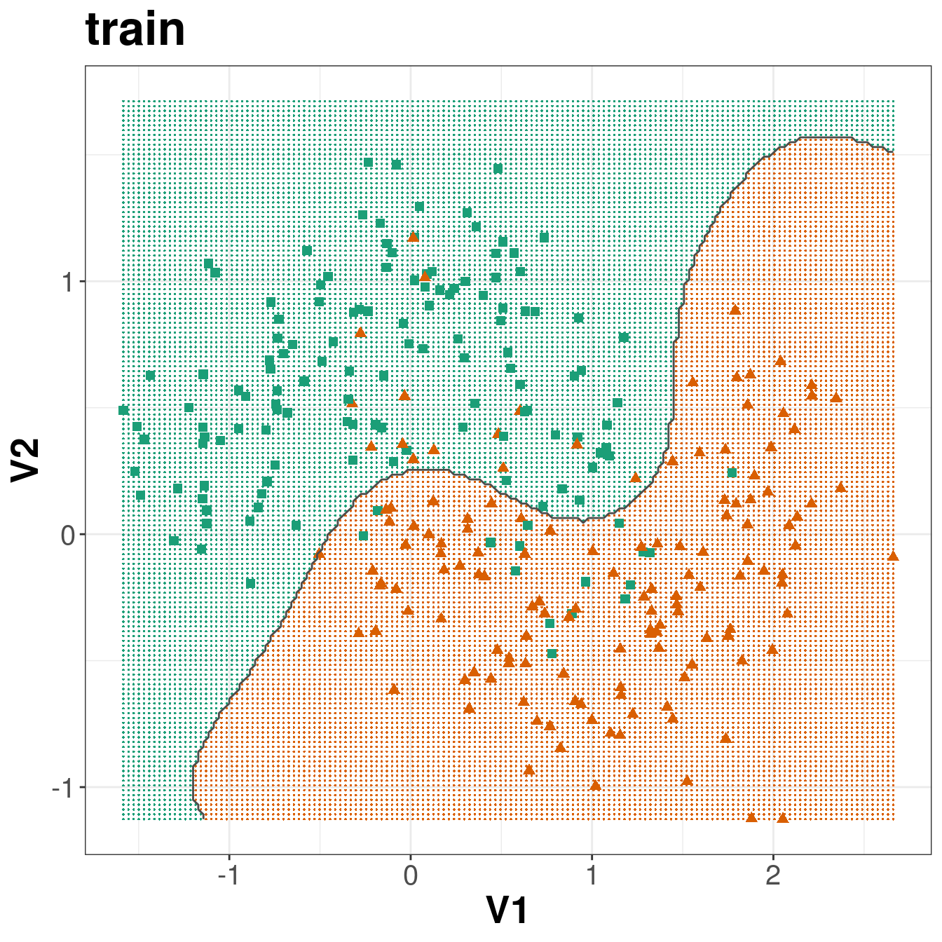
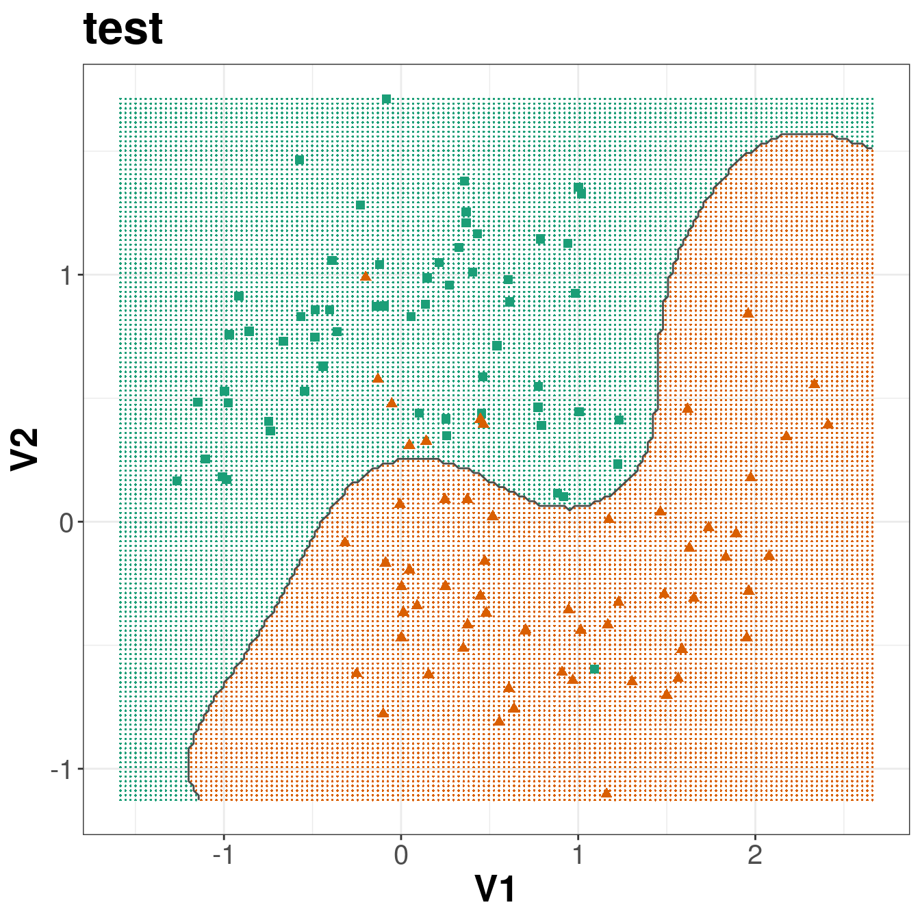
Figure 6.12: Decision boundary created by radial kernel SVM.
6.5 Defining your own model type to use in caret
Caret has over two hundred built in models, including several support vector machines: https://topepo.github.io/caret/available-models.html
However, despite this wide range of options, you may occasionally need to define your own model. Caret does not currently have a radial SVM implemented using the e1071 library, so we will define one here.
svmRadialE1071 <- list(
  label = "Support Vector Machines with Radial Kernel - e1071",
  library = "e1071",
  type = c("Regression", "Classification"),
  parameters = data.frame(parameter="cost",
                          class="numeric",
                          label="Cost"),
  grid = function (x, y, len = NULL, search = "grid")
    {
      if (search == "grid") {
        out <- expand.grid(cost = 2^((1:len) - 3))
      }
      else {
        out <- data.frame(cost = 2^runif(len, min = -5, max = 10))
      }
      out
    },
  loop=NULL,
  fit=function (x, y, wts, param, lev, last, classProbs, ...)
    {
      if (any(names(list(...)) == "probability") | is.numeric(y)) {
        out <- e1071::svm(x = as.matrix(x), y = y, kernel = "radial",
                          cost = param$cost, ...)
      }
      else {
        out <- e1071::svm(x = as.matrix(x), y = y, kernel = "radial",
                          cost = param$cost, probability = classProbs, ...)
      }
      out
    },
  predict = function (modelFit, newdata, submodels = NULL)
    {
      predict(modelFit, newdata)
    },
  prob = function (modelFit, newdata, submodels = NULL)
    {
      out <- predict(modelFit, newdata, probability = TRUE)
      attr(out, "probabilities")
    },
  predictors = function (x, ...)
    {
      out <- if (!is.null(x$terms))
        predictors.terms(x$terms)
      else x$xNames
      if (is.null(out))
        out <- names(attr(x, "scaling")$x.scale$`scaled:center`)
      if (is.null(out))
        out <- NA
      out
    },
  tags = c("Kernel Methods", "Support Vector Machines", "Regression", "Classifier", "Robust Methods"),
  levels = function(x) x$levels,
  sort = function(x)
  {
    x[order(x$cost), ]
  }
)
Note that the radial SVM model we have defined has only one tuning parameter, cost (C). If we do not define the kernel parameter gamma, e1071 will automatically calculate it as 1/(data dimension); i.e. if we have 58 predictors, gamma will be 1/58 = 0.01724.
6.5.1 Model cross-validation and tuning
We will pass the twoClassSummary function into model training through trainControl. Additionally we would like the model to predict class probabilities so that we can calculate the ROC curve, so we use the classProbs option.
cvCtrl <- trainControl(method = "repeatedcv",
                       repeats = 10,
                       number = 10,
                       summaryFunction = twoClassSummary,
                       classProbs = TRUE,
                       seeds=seeds)
We set the method of the train function to svmRadial to specify a radial kernel SVM. In this implementation we only have to tune one parameter, cost. The default grid of cost parameters start at 0.25 and double at each iteration. Choosing tuneLength = 9 will give us cost parameters of 0.25, 0.5, 1, 2, 4, 8, 16, 32 and 64.
svmTune <- train(x = moonsTrain[,c(1:2)],
                 y = moonsTrain[,3],
                 method = svmRadialE1071,
                 tuneLength = 9,
                 preProc = c("center", "scale"),
                 metric = "ROC",
                 trControl = cvCtrl)

svmTune
## Support Vector Machines with Radial Kernel - e1071
##
## 280 samples
## 2 predictor
## 2 classes: 'A', 'B'
##
## Pre-processing: centered (2), scaled (2)
## Resampling: Cross-Validated (10 fold, repeated 10 times)
## Summary of sample sizes: 252, 252, 252, 252, 252, 252, ...
## Resampling results across tuning parameters:
##
## cost ROC Sens Spec
## 0.25 0.9230612 0.8378571 0.9057143
## 0.50 0.9320918 0.8592857 0.9057143
## 1.00 0.9418878 0.8692857 0.9000000
## 2.00 0.9455102 0.8792857 0.8964286
## 4.00 0.9479082 0.8785714 0.8914286
## 8.00 0.9485204 0.8678571 0.8857143
## 16.00 0.9492857 0.8757143 0.8800000
## 32.00 0.9490816 0.8764286 0.8728571
## 64.00 0.9463776 0.8778571 0.8707143
##
## ROC was used to select the optimal model using the largest value.
## The final value used for the model was cost = 16.svmTune$finalModel##
## Call:
## svm.default(x = as.matrix(x), y = y, kernel = "radial", cost = param$cost,
## probability = classProbs)
##
##
## Parameters:
## SVM-Type: C-classification
## SVM-Kernel: radial
## cost: 16
##
## Number of Support Vectors: 796.6 Iris example
library(datasets)
data(iris) ##loads the dataset, which can be accessed under the variable name iris
?iris ##opens the documentation for the dataset
summary(iris) ##presents the 5 figure summary of the dataset
## Sepal.Length Sepal.Width Petal.Length Petal.Width
## Min. :4.300 Min. :2.000 Min. :1.000 Min. :0.100
## 1st Qu.:5.100 1st Qu.:2.800 1st Qu.:1.600 1st Qu.:0.300
## Median :5.800 Median :3.000 Median :4.350 Median :1.300
## Mean :5.843 Mean :3.057 Mean :3.758 Mean :1.199
## 3rd Qu.:6.400 3rd Qu.:3.300 3rd Qu.:5.100 3rd Qu.:1.800
## Max. :7.900 Max. :4.400 Max. :6.900 Max. :2.500
## Species
## setosa :50
## versicolor:50
## virginica :50
##
##
## str(iris) ##presents the structure of the iris dataframe## 'data.frame': 150 obs. of 5 variables:
## $ Sepal.Length: num 5.1 4.9 4.7 4.6 5 5.4 4.6 5 4.4 4.9 ...
## $ Sepal.Width : num 3.5 3 3.2 3.1 3.6 3.9 3.4 3.4 2.9 3.1 ...
## $ Petal.Length: num 1.4 1.4 1.3 1.5 1.4 1.7 1.4 1.5 1.4 1.5 ...
## $ Petal.Width : num 0.2 0.2 0.2 0.2 0.2 0.4 0.3 0.2 0.2 0.1 ...
## $ Species : Factor w/ 3 levels "setosa","versicolor",..: 1 1 1 1 1 1 1 1 1 1 ...set.seed(42)
trainTestPartition<-createDataPartition(y=iris$Species, #the class label, caret ensures an even split of classes
p=0.7, #proportion of samples assigned to train
list=FALSE)
str(trainTestPartition)## int [1:105, 1] 1 2 3 4 5 7 8 10 11 12 ...
## - attr(*, "dimnames")=List of 2
## ..$ : NULL
## ..$ : chr "Resample1"iris.training <- iris[ trainTestPartition,] #take the corresponding rows for training
iris.testing <- iris[-trainTestPartition,] #take the corresponding rows for testing by removing training rowsset.seed(42)
seeds = vector(mode='list',length=101) #you need length #folds*#repeats + 1 so 10*10 + 1 here
for (i in 1:100) seeds[[i]] = sample.int(1000,10)
seeds[[101]] = sample.int(1000,1)
train_ctrl_seed_repeated = trainControl(method='repeatedcv',
number=10, #number of folds
repeats=10, #number of times to repeat cross-validation
seeds=seeds)
iris_svm <- train(
Species ~ .,
data = iris.training,
method = "svmLinear",
parms = list(split = "gini"),
preProc = c("corr","nzv","center", "scale","BoxCox"),
tuneLength=10,
trControl = train_ctrl_seed_repeated
)
iris_svm## Support Vector Machines with Linear Kernel
##
## 105 samples
## 4 predictor
## 3 classes: 'setosa', 'versicolor', 'virginica'
##
## Pre-processing: centered (3), scaled (3), Box-Cox transformation (3), remove (1)
## Resampling: Cross-Validated (10 fold, repeated 10 times)
## Summary of sample sizes: 94, 95, 94, 93, 95, 95, ...
## Resampling results:
##
## Accuracy Kappa
## 0.9740152 0.9605099
##
## Tuning parameter 'C' was held constant at a value of 1iris_information_predict_train=predict(iris_svm,iris.training,type='raw')
confusionMatrix(iris_information_predict_train,iris.training$Species)## Confusion Matrix and Statistics
##
## Reference
## Prediction setosa versicolor virginica
## setosa 35 0 0
## versicolor 0 35 2
## virginica 0 0 33
##
## Overall Statistics
##
## Accuracy : 0.981
## 95% CI : (0.9329, 0.9977)
## No Information Rate : 0.3333
## P-Value [Acc > NIR] : < 2.2e-16
##
## Kappa : 0.9714
##
## Mcnemar's Test P-Value : NA
##
## Statistics by Class:
##
## Class: setosa Class: versicolor Class: virginica
## Sensitivity 1.0000 1.0000 0.9429
## Specificity 1.0000 0.9714 1.0000
## Pos Pred Value 1.0000 0.9459 1.0000
## Neg Pred Value 1.0000 1.0000 0.9722
## Prevalence 0.3333 0.3333 0.3333
## Detection Rate 0.3333 0.3333 0.3143
## Detection Prevalence 0.3333 0.3524 0.3143
## Balanced Accuracy 1.0000 0.9857 0.9714iris_gini_predict=predict(iris_svm,iris.testing,type='raw')
confusionMatrix(iris_gini_predict,iris.testing$Species)## Confusion Matrix and Statistics
##
## Reference
## Prediction setosa versicolor virginica
## setosa 15 0 0
## versicolor 0 13 2
## virginica 0 2 13
##
## Overall Statistics
##
## Accuracy : 0.9111
## 95% CI : (0.7878, 0.9752)
## No Information Rate : 0.3333
## P-Value [Acc > NIR] : 8.467e-16
##
## Kappa : 0.8667
##
## Mcnemar's Test P-Value : NA
##
## Statistics by Class:
##
## Class: setosa Class: versicolor Class: virginica
## Sensitivity 1.0000 0.8667 0.8667
## Specificity 1.0000 0.9333 0.9333
## Pos Pred Value 1.0000 0.8667 0.8667
## Neg Pred Value 1.0000 0.9333 0.9333
## Prevalence 0.3333 0.3333 0.3333
## Detection Rate 0.3333 0.2889 0.2889
## Detection Prevalence 0.3333 0.3333 0.3333
## Balanced Accuracy 1.0000 0.9000 0.90006.7 Cell segmentation example
Load required libraries
library(caret)
library(pROC)
library(e1071)
Load data
data(segmentationData)segClass <- segmentationData$ClassExtract predictors from segmentationData
segData <- segmentationData[,4:59]Partition data
set.seed(42)
trainIndex <- createDataPartition(y=segClass, times=1, p=0.5, list=F)
segDataTrain <- segData[trainIndex,]
segDataTest <- segData[-trainIndex,]
segClassTrain <- segClass[trainIndex]
segClassTest <- segClass[-trainIndex]
Set seeds for reproducibility (optional). We will be trying 9 values of the tuning parameter with 5 repeats of 10 fold cross-validation, so we need the following list of seeds.
set.seed(42)
seeds <- vector(mode = "list", length = 51)
for(i in 1:50) seeds[[i]] <- sample.int(1000, 9)
seeds[[51]] <- sample.int(1000,1)
We will pass the twoClassSummary function into model training through trainControl. Additionally we would like the model to predict class probabilities so that we can calculate the ROC curve, so we use the classProbs option.
cvCtrl <- trainControl(method = "repeatedcv",
                       repeats = 5,
                       number = 10,
                       summaryFunction = twoClassSummary,
                       classProbs = TRUE,
                       seeds=seeds)
Tune SVM over the cost parameter. The default grid of cost parameters start at 0.25 and double at each iteration. Choosing tuneLength = 9 will give us cost parameters of 0.25, 0.5, 1, 2, 4, 8, 16, 32 and 64. The train function will calculate an appropriate value of sigma (the kernel parameter) from the data.
svmTune <- train(x = segDataTrain,
                 y = segClassTrain,
                 method = 'svmRadial',
                 tuneLength = 9,
                 preProc = c("center", "scale"),
                 metric = "ROC",
                 trControl = cvCtrl)

svmTune
## Support Vector Machines with Radial Basis Function Kernel
##
## 1010 samples
## 56 predictor
## 2 classes: 'PS', 'WS'
##
## Pre-processing: centered (56), scaled (56)
## Resampling: Cross-Validated (10 fold, repeated 5 times)
## Summary of sample sizes: 909, 909, 909, 909, 909, 909, ...
## Resampling results across tuning parameters:
##
## C ROC Sens Spec
## 0.25 0.8767949 0.8636923 0.6916667
## 0.50 0.8820256 0.8769231 0.6955556
## 1.00 0.8820855 0.8812308 0.7072222
## 2.00 0.8805983 0.8787692 0.7105556
## 4.00 0.8741538 0.8756923 0.6905556
## 8.00 0.8600085 0.8695385 0.6694444
## 16.00 0.8472393 0.8732308 0.6477778
## 32.00 0.8369231 0.8769231 0.6144444
## 64.00 0.8246496 0.8661538 0.6133333
##
## Tuning parameter 'sigma' was held constant at a value of 0.01598045
## ROC was used to select the optimal model using the largest value.
## The final values used for the model were sigma = 0.01598045 and C = 1.svmTune$finalModel## Support Vector Machine object of class "ksvm"
##
## SV type: C-svc (classification)
## parameter : cost C = 1
##
## Gaussian Radial Basis kernel function.
## Hyperparameter : sigma = 0.0159804470403774
##
## Number of Support Vectors : 537
##
## Objective Function Value : -388.0962
## Training error : 0.132673
## Probability model included.SVM accuracy profile
plot(svmTune, metric = "ROC", scales = list(x = list(log =2)))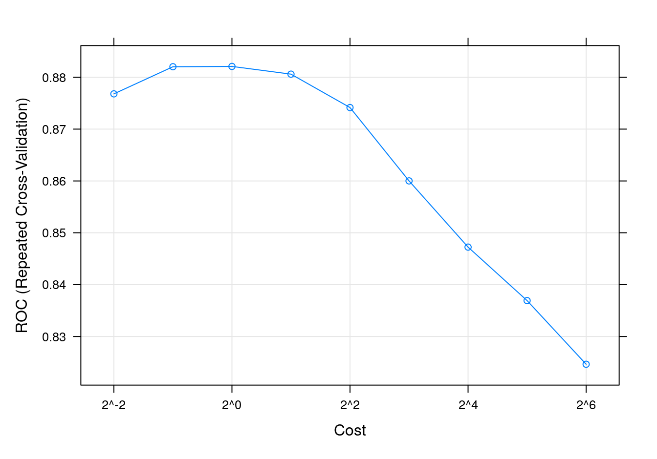
Figure 6.13: SVM accuracy profile.
Test set results
svmPred <- predict(svmTune, segDataTest)
confusionMatrix(svmPred, segClassTest)
## Confusion Matrix and Statistics
##
## Reference
## Prediction PS WS
## PS 578 111
## WS 72 248
##
## Accuracy : 0.8186
## 95% CI : (0.7934, 0.8419)
## No Information Rate : 0.6442
## P-Value [Acc > NIR] : < 2.2e-16
##
## Kappa : 0.5945
##
## Mcnemar's Test P-Value : 0.004969
##
## Sensitivity : 0.8892
## Specificity : 0.6908
## Pos Pred Value : 0.8389
## Neg Pred Value : 0.7750
## Prevalence : 0.6442
## Detection Rate : 0.5728
## Detection Prevalence : 0.6829
## Balanced Accuracy : 0.7900
##
## 'Positive' Class : PS
## Get predicted class probabilities
svmProbs <- predict(svmTune, segDataTest, type="prob")
head(svmProbs)
## PS WS
## 1 0.9015892 0.09841085
## 2 0.9127814 0.08721855
## 3 0.9699164 0.03008361
## 4 0.5828048 0.41719516
## 5 0.8283722 0.17162781
## 6 0.7702593 0.22974067Build a ROC curve
svmROC <- roc(segClassTest, svmProbs[,"PS"])## Setting levels: control = PS, case = WS## Setting direction: controls > casesauc(svmROC)## Area under the curve: 0.8912Plot ROC curve.
plot(svmROC, type = "S")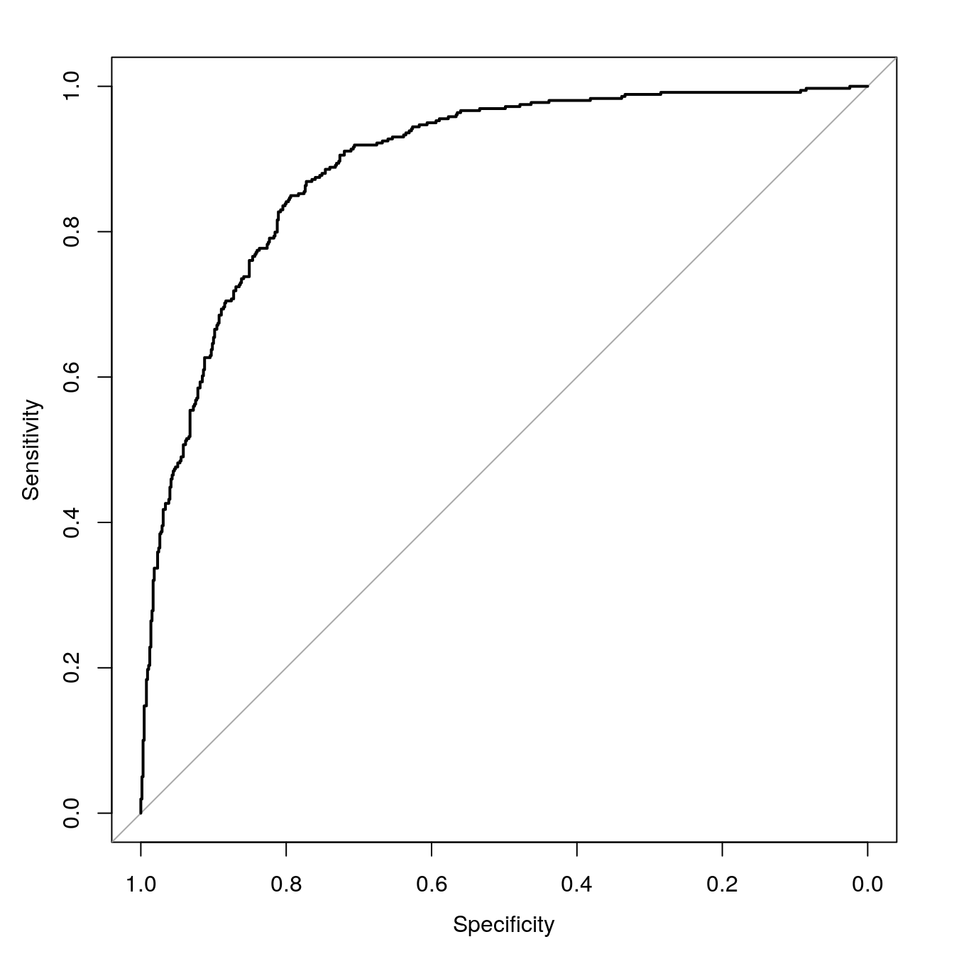
Figure 6.14: SVM ROC curve for cell segmentation data set.
Calculate area under ROC curve
auc(svmROC)## Area under the curve: 0.89126.8 Example - regression
This example serves to demonstrate the use of SVMs in regression, but perhaps more importantly, it highlights the power and flexibility of the caret package. Earlier we used k-NN for a regression analysis of the BloodBrain dataset (see section 04-nearest-neighbours.Rmd). We will repeat the regression analysis, but this time we will fit a radial kernel SVM. Remarkably, a re-run of this analysis using a completely different type of model, requires changes to only two lines of code.
The pre-processing steps and generation of seeds are identical, therefore if the data were still in memory, we could skip this next block of code:
data(BloodBrain)

set.seed(42)
trainIndex <- createDataPartition(y=logBBB, times=1, p=0.8, list=F)
descrTrain <- bbbDescr[trainIndex,]
concRatioTrain <- logBBB[trainIndex]
descrTest <- bbbDescr[-trainIndex,]
concRatioTest <- logBBB[-trainIndex]

transformations <- preProcess(descrTrain,
                              method=c("center", "scale", "corr", "nzv"),
                              cutoff=0.75)
descrTrain <- predict(transformations, descrTrain)

set.seed(42)
seeds <- vector(mode = "list", length = 26)
for(i in 1:25) seeds[[i]] <- sample.int(1000, 50)
seeds[[26]] <- sample.int(1000,1)
In the arguments to the train function we change method from knn to svmRadialE1071. The tunegrid parameter is replaced with tuneLength = 9. Now we are ready to fit an SVM model.
svmTune2 <- train(descrTrain,
                 concRatioTrain,
                 method=svmRadialE1071,
                 tuneLength = 9,
                 trControl = trainControl(method="repeatedcv",
                                          number = 5,
                                          repeats = 5,
                                          seeds=seeds
                                          )
)

svmTune2
## Support Vector Machines with Radial Kernel - e1071
##
## 168 samples
## 63 predictor
##
## No pre-processing
## Resampling: Cross-Validated (5 fold, repeated 5 times)
## Summary of sample sizes: 136, 134, 134, 134, 134, 134, ...
## Resampling results across tuning parameters:
##
## cost RMSE Rsquared MAE
## 0.25 0.6161239 0.4980242 0.4610789
## 0.50 0.5734394 0.5332846 0.4316062
## 1.00 0.5465607 0.5505891 0.4178574
## 2.00 0.5300490 0.5661867 0.4035017
## 4.00 0.5248272 0.5712901 0.3985361
## 8.00 0.5244977 0.5718310 0.3980940
## 16.00 0.5244977 0.5718310 0.3980940
## 32.00 0.5244977 0.5718310 0.3980940
## 64.00 0.5244977 0.5718310 0.3980940
##
## RMSE was used to select the optimal model using the smallest value.
## The final value used for the model was cost = 8.plot(svmTune2)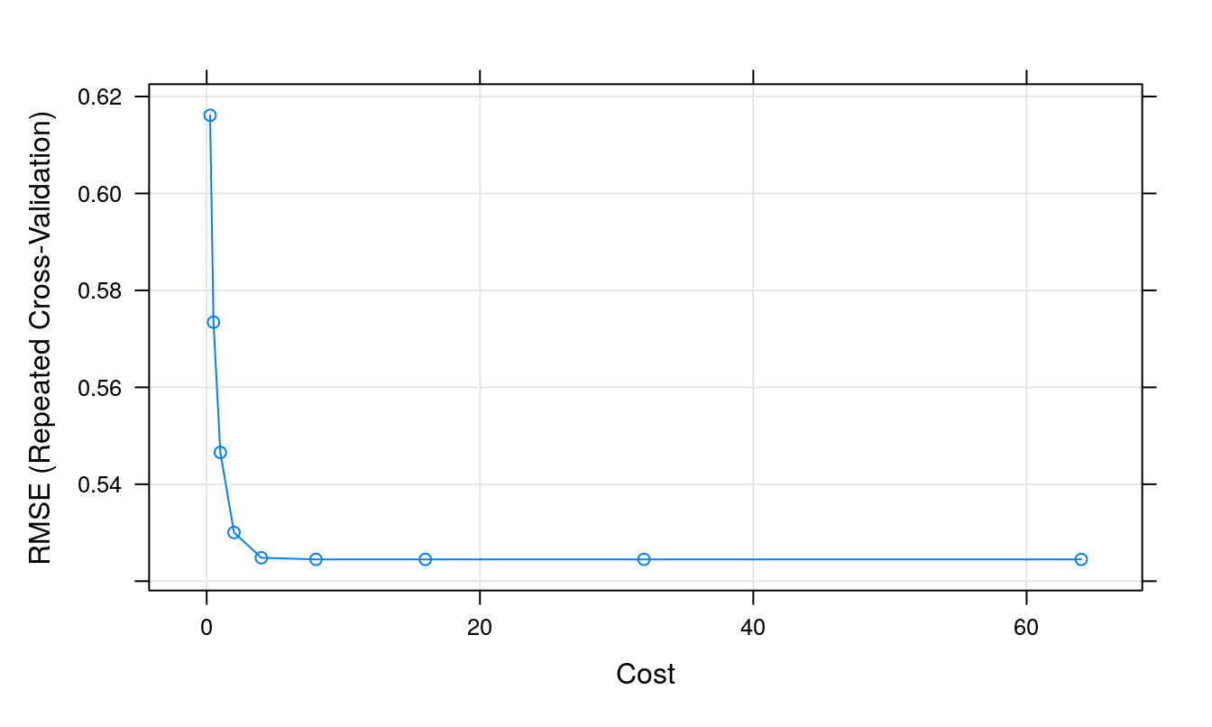
Figure 6.15: Root Mean Squared Error as a function of cost.
Use model to predict outcomes, after first pre-processing the test set.
descrTest <- predict(transformations, descrTest)
test_pred <- predict(svmTune2, descrTest)
Prediction performance can be visualized in a scatterplot.
qplot(concRatioTest, test_pred) +
  xlab("observed") +
  ylab("predicted") +
  theme_bw()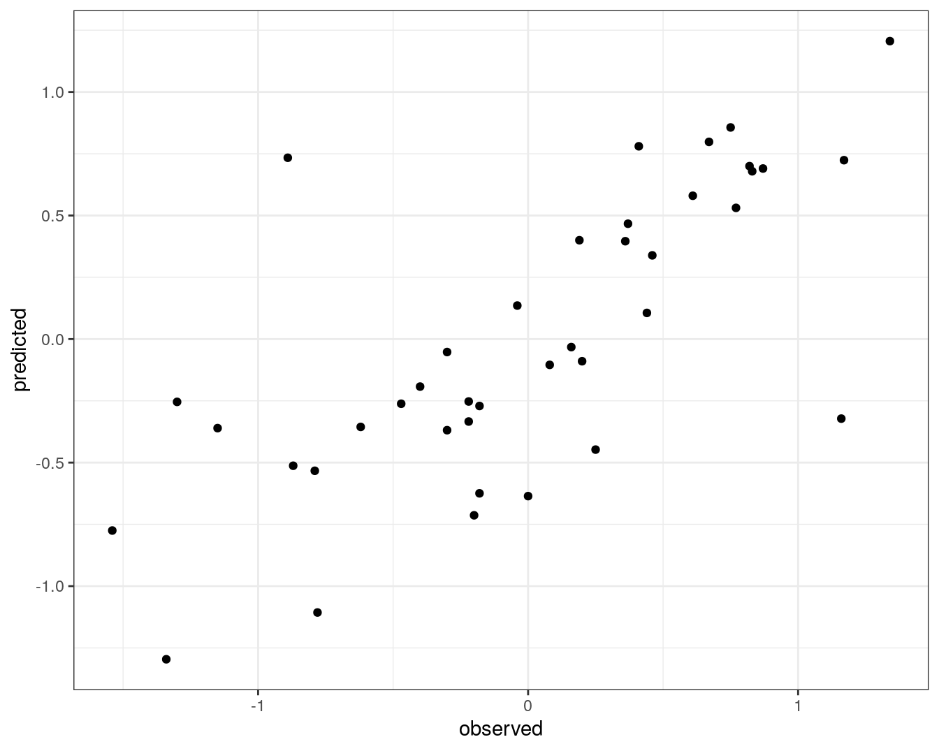
Figure 6.16: Concordance between observed concentration ratios and those predicted by radial kernel SVM.
We can also measure correlation between observed and predicted values.
cor(concRatioTest, test_pred)## [1] 0.7274762