B Solutions - Dimensionality reduction

Solutions to exercises of dimensionality reduction chapter.

B.1 Exercise 1.

Read in the corresponding spreadsheet into the R environment as a data frame variable.

library(tidyverse)
set.seed(12345)

sc_rna <- read_csv(file = "data/PGC_transcriptomics/PGC_transcriptomics.csv")

metadata <- sc_rna %>% 
  slice( 1:4) %>% 
  pivot_longer( cols=-Sample, names_to = 'cell_type', values_to  = 'index') %>% 
  pivot_wider( names_from = Sample, values_from = index) %>% 
  mutate(group=str_remove(cell_type, '\\..*$')) %>% 
  mutate_if( is.numeric, as.factor)  
  
sc_rna_fil <- sc_rna %>% 
  slice(-c(1:4)) %>% 
  column_to_rownames(var='Sample') %>% 
  as.matrix()

genenames <- rownames(sc_rna_fil)
cell_type <- colnames(sc_rna_fil) 

We can run tSNE using the following command:

library(Rtsne)
set.seed(1)
tsne_model_1 = Rtsne(as.matrix(t(sc_rna_fil)), check_duplicates=FALSE, pca=TRUE, perplexity=100, theta=0.5, dims=2)

As we did previously, we can plot the results using:

sc_2d_data <- tsne_model_1$Y %>% 
  as.data.frame() %>% 
  rename( x=V1,y=V2) %>% 
  mutate(cell_type = cell_type ) %>% 
  mutate( cell_group = str_remove(cell_type, '\\..*$'))

ggplot(data=sc_2d_data) +
  geom_point( mapping=aes(x=x,y=y, color=cell_group), alpha=0.5) +
  scale_x_continuous(limits = c(-20,20)) +
  scale_y_continuous(limits = c(-20,20)) +
  theme_classic()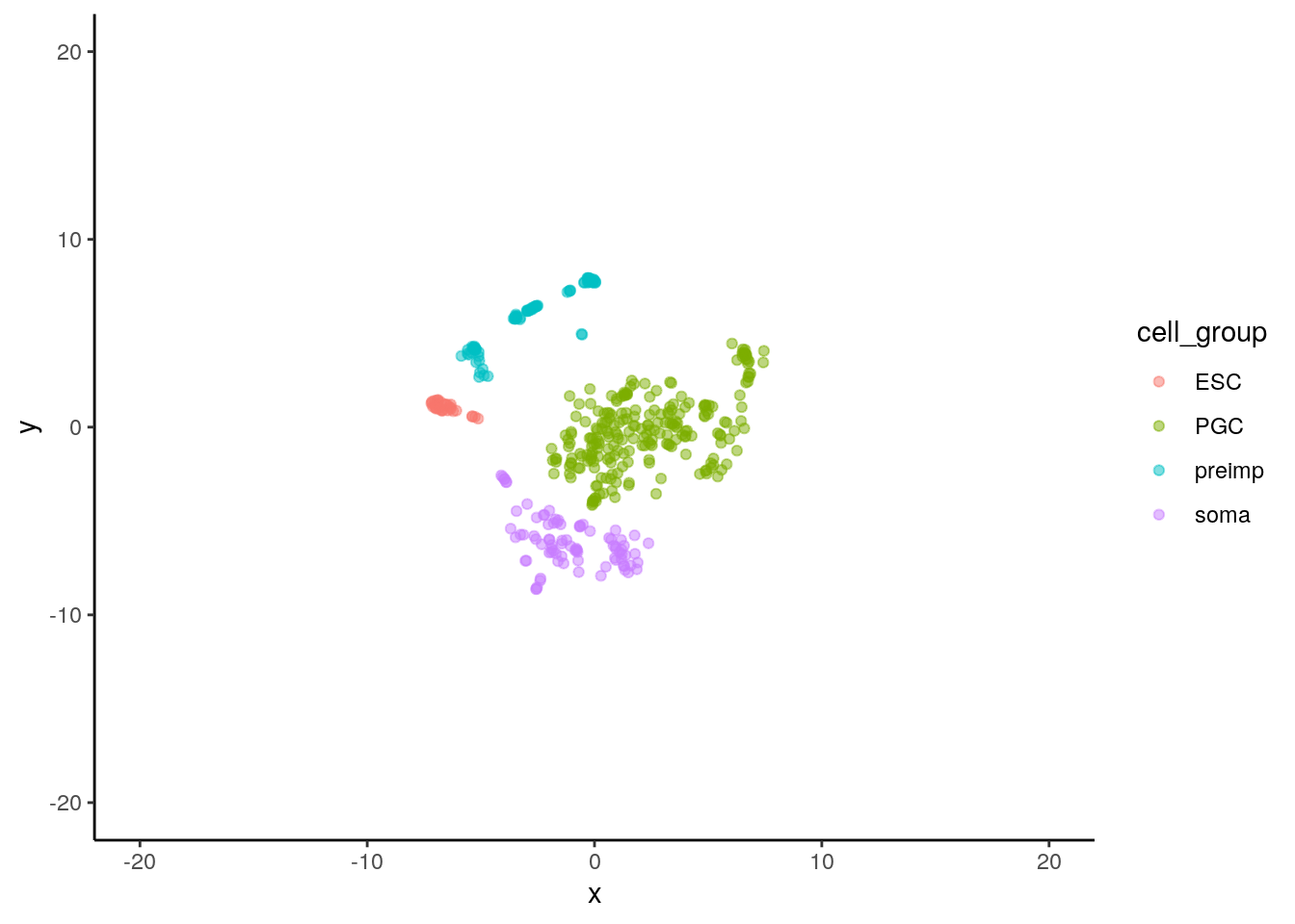

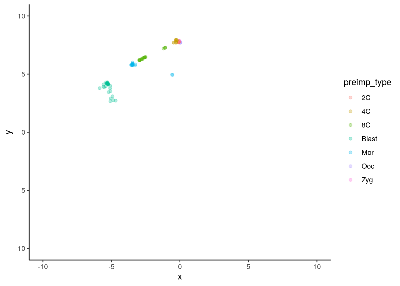
B.2 Exercise 2.

We can plot the expression patterns for pre-implantation embryos:

sc_2d_preimp <- inner_join(sc_2d_data, metadata, by='cell_type') %>% 
  filter(cell_group  == 'preimp') %>% 
  mutate( preimp_type = recode(as.character(Time), 
                       '0' = 'Ooc',
                       '1' = 'Zyg',
                       '2' = '2C',
                       '3' = '4C',
                       '4'  = '8C',
                       '5' = 'Mor',
                       '6' = 'Blast'))

ggplot(data=sc_2d_preimp) +
  geom_point( mapping = aes(x=x,  y=y, color=preimp_type), alpha=0.3) +
  scale_x_continuous(limits = c(-10,10)) +
  scale_y_continuous(limits = c(-10,10)) +
  theme_classic()