D Solutions ch. 7 - Nearest neighbours
Solutions to exercises of chapter 5.
D.1 Exercise 1
Load libraries
library(caret)## Loading required package: ggplot2## Loading required package: lattice## Warning in system("timedatectl", intern = TRUE): running command 'timedatectl'
## had status 1library(RColorBrewer)
library(doMC)## Loading required package: foreach## Loading required package: iterators## Loading required package: parallellibrary(corrplot)## corrplot 0.92 loadedPrepare for parallel processing
registerDoMC(detectCores())Load data
load("data/wheat_seeds/wheat_seeds.Rda")Partition data
set.seed(42)
trainIndex <- createDataPartition(y=variety, times=1, p=0.7, list=F)
varietyTrain <- variety[trainIndex]
morphTrain <- morphometrics[trainIndex,]
varietyTest <- variety[-trainIndex]
morphTest <- morphometrics[-trainIndex,]

summary(varietyTrain)
## Canadian Kama Rosa
## 49 49 49summary(varietyTest)## Canadian Kama Rosa
## 21 21 21Data check: zero and near-zero predictors
nzv <- nearZeroVar(morphTrain, saveMetrics=T)
nzv
## freqRatio percentUnique zeroVar nzv
## area 1.500000 95.91837 FALSE FALSE
## perimeter 1.333333 86.39456 FALSE FALSE
## compactness 1.000000 91.83673 FALSE FALSE
## kernLength 1.000000 91.15646 FALSE FALSE
## kernWidth 1.000000 91.83673 FALSE FALSE
## asymCoef 2.000000 99.31973 FALSE FALSE
## grooveLength 1.333333 76.19048 FALSE FALSEData check: are all predictors on same scale?
summary(morphTrain)## area perimeter compactness kernLength
## Min. :10.59 Min. :12.41 Min. :0.8081 Min. :4.899
## 1st Qu.:12.34 1st Qu.:13.46 1st Qu.:0.8577 1st Qu.:5.264
## Median :14.46 Median :14.40 Median :0.8734 Median :5.541
## Mean :14.87 Mean :14.56 Mean :0.8724 Mean :5.624
## 3rd Qu.:17.10 3rd Qu.:15.65 3rd Qu.:0.8881 3rd Qu.:5.979
## Max. :20.97 Max. :17.25 Max. :0.9153 Max. :6.675
## kernWidth asymCoef grooveLength
## Min. :2.630 Min. :0.903 Min. :4.519
## 1st Qu.:2.958 1st Qu.:2.372 1st Qu.:5.046
## Median :3.259 Median :3.597 Median :5.222
## Mean :3.267 Mean :3.659 Mean :5.406
## 3rd Qu.:3.557 3rd Qu.:4.799 3rd Qu.:5.862
## Max. :4.032 Max. :8.456 Max. :6.550featurePlot(x = morphTrain,
y = varietyTrain,
plot = "box",
## Pass in options to bwplot()
scales = list(y = list(relation="free"),
x = list(rot = 90)),
layout = c(3,3))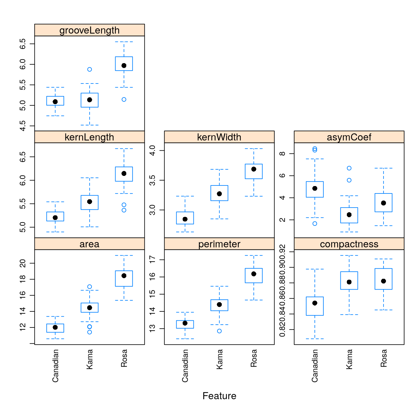
Figure D.1: Boxplots of the 7 geometric parameters in the wheat data set
Data check: pairwise correlations between predictors
corMat <- cor(morphTrain)
corrplot(corMat, order="hclust", tl.cex=1)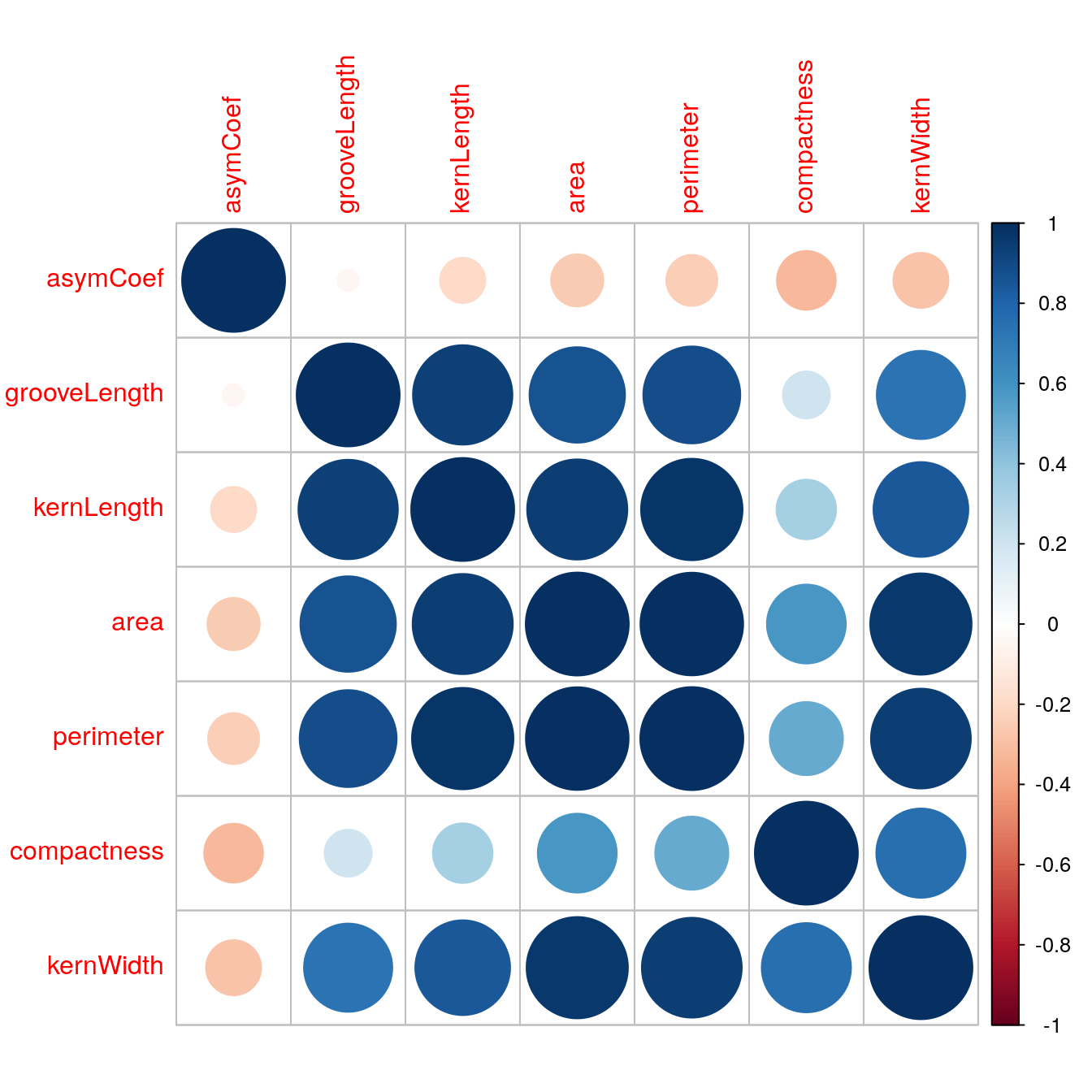
Figure D.2: Correlogram of the wheat seed data set.
highCorr <- findCorrelation(corMat, cutoff=0.75)
length(highCorr)
## [1] 4names(morphTrain)[highCorr]## [1] "area" "perimeter" "kernWidth" "kernLength"Data check: skewness
featurePlot(x = morphTrain,
            y = varietyTrain,
            plot = "density",
            ## Pass in options to xyplot() to
            ## make it prettier
            scales = list(x = list(relation="free"),
                          y = list(relation="free")),
            adjust = 1.5,
            pch = "|",
            layout = c(3, 3),
            auto.key = list(columns = 3))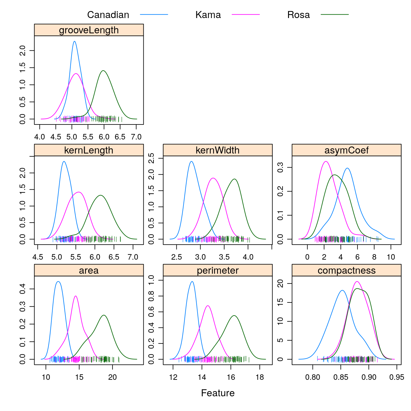
Figure D.3: Density plots of the 7 geometric parameters in the wheat data set
Create a ‘grid’ of values of k for evaluation:
tuneParam <- data.frame(k=seq(1,50,2))Generate a list of seeds for reproducibility (optional) based on grid size
set.seed(42)
seeds <- vector(mode = "list", length = 101)
for(i in 1:100) seeds[[i]] <- sample.int(1000, length(tuneParam$k))
seeds[[101]] <- sample.int(1000,1)
Set training parameters. In the example in chapter 5 pre-processing was performed outside the cross-validation process to save time for the purposes of the demonstration. Here we have a relatively small data set, so we can do pre-processing within each iteration of the cross-validation process. We specify the option preProcOptions=list(cutoff=0.75) to set a value for the pairwise correlation coefficient cutoff.
train_ctrl <- trainControl(method="repeatedcv",
                   number = 10,
                   repeats = 10,
                   preProcOptions=list(cutoff=0.75),
                   seeds = seeds)
Run training
knnFit <- train(morphTrain, varietyTrain,
                method="knn",
                preProcess = c("center", "scale", "corr"),
                tuneGrid=tuneParam,
                trControl=train_ctrl)
knnFit
## k-Nearest Neighbors
##
## 147 samples
## 7 predictor
## 3 classes: 'Canadian', 'Kama', 'Rosa'
##
## Pre-processing: centered (3), scaled (3), remove (4)
## Resampling: Cross-Validated (10 fold, repeated 10 times)
## Summary of sample sizes: 133, 132, 133, 132, 132, 133, ...
## Resampling results across tuning parameters:
##
## k Accuracy Kappa
## 1 0.8640238 0.7955794
## 3 0.8411667 0.7614211
## 5 0.8544524 0.7813197
## 7 0.8646429 0.7966349
## 9 0.8743810 0.8111795
## 11 0.8771429 0.8154320
## 13 0.8777619 0.8162978
## 15 0.8804762 0.8204404
## 17 0.8852857 0.8276139
## 19 0.8839048 0.8255536
## 21 0.8846190 0.8266306
## 23 0.8846190 0.8266223
## 25 0.8839048 0.8255454
## 27 0.8853333 0.8277076
## 29 0.8908095 0.8359544
## 31 0.8907619 0.8358447
## 33 0.8921429 0.8379874
## 35 0.8874762 0.8309461
## 37 0.8894762 0.8339626
## 39 0.8888095 0.8329793
## 41 0.8880952 0.8319026
## 43 0.8880476 0.8317839
## 45 0.8907619 0.8358610
## 47 0.8874286 0.8308694
## 49 0.8866667 0.8297155
##
## Accuracy was used to select the optimal model using the largest value.
## The final value used for the model was k = 33.Plot cross validation accuracy as a function of k
plot(knnFit)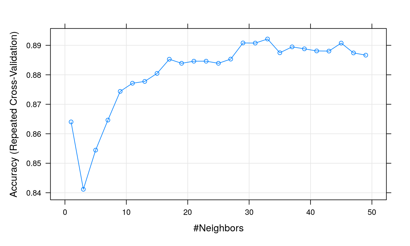
Figure D.4: Accuracy (repeated cross-validation) as a function of neighbourhood size for the wheat seeds data set.
Predict the class (wheat variety) of the observations in the test set.
test_pred <- predict(knnFit, morphTest)
confusionMatrix(test_pred, varietyTest)
## Confusion Matrix and Statistics
##
## Reference
## Prediction Canadian Kama Rosa
## Canadian 20 3 0
## Kama 1 17 0
## Rosa 0 1 21
##
## Overall Statistics
##
## Accuracy : 0.9206
## 95% CI : (0.8244, 0.9737)
## No Information Rate : 0.3333
## P-Value [Acc > NIR] : < 2.2e-16
##
## Kappa : 0.881
##
## Mcnemar's Test P-Value : NA
##
## Statistics by Class:
##
## Class: Canadian Class: Kama Class: Rosa
## Sensitivity 0.9524 0.8095 1.0000
## Specificity 0.9286 0.9762 0.9762
## Pos Pred Value 0.8696 0.9444 0.9545
## Neg Pred Value 0.9750 0.9111 1.0000
## Prevalence 0.3333 0.3333 0.3333
## Detection Rate 0.3175 0.2698 0.3333
## Detection Prevalence 0.3651 0.2857 0.3492
## Balanced Accuracy 0.9405 0.8929 0.9881