2 Introduction
In the era of large scale data collection we are trying to make meaningful intepretation of data.
There are two ways to meaningfully intepret data and they are
- Mechanistic or mathematical modeling based
- Descriptive or Data Driven
We are here to discuss the later approach using machine learning (ML) approaches.
2.1 What is machine learning?
We use - computers - more precisely - algorithms to see patterns and learn concepts from data - without being explicitly programmed.
For example
- Google ranking web pages
- Facebook or Gmail classifying Spams
- Biological research projects that we are doing - we use ML approaches to interpret effects of mutations in the noncoding regions.
We are given a set of
- Predictors
- Features or
- Inputs
that we call ‘Explanatory Variables’
and we ask different statistical methods, such as
- Linear Regression
- Logistic Regression
- Neural Networks
to formulate an hypothesis i.e.
- Describe associations
- Search for patterns
- Make predictions
for the Outcome Variables
A bit of a background: ML grew out of AI and Neural Networks
2.2 Aspects of ML
There are two aspects of ML
- Unsupervised learning
- Supervised learning
Unsupervised learning: When we ask an algorithm to find patterns or structure in the data without any specific outcome variables e.g. clustering. We have little or no idea how the results should look like.
Supervised learning: When we give both input and outcome variables and we ask the algorithm to formulate an hypothesis that closely captures the relationship.
2.3 What actually happened under the hood
The algorithms take a subset of observations called as the training data and tests them on a different subset of data called as the test data.
The error between the prediction of the outcome variable the actual data is evaulated as test error. The objective function of the algorithm is to minimise these test errors by tuning the parameters of the hypothesis.
Models that successfully capture these desired outcomes are further evaluated for Bias and Variance (overfitting and underfitting).
All the above concepts will be discussed in detail in the following lectures.
2.4 Introduction to CARET
The caret package (short for Classification And REgression Training) contains functions to streamline the model training process for classification and regression tasks.
library(caret)## Loading required package: ggplot2## Loading required package: lattice## Warning in system("timedatectl", intern = TRUE): running command 'timedatectl'
## had status 12.4.1 Preprocessing with the Iris dataset
From the iris manual page:
The famous (Fisher’s or Anderson’s) Iris data set, first presented by Fisher in 1936 (http://archive.ics.uci.edu/ml/datasets/Iris), gives the measurements in centimeters of the variables sepal length and width and petal length and width, respectively, for 50 flowers from each of 3 species of iris. The species are Iris setosa, versicolor, and virginica. One class is linearly separable from the other two; the latter are not linearly separable from each other. The data base contains the following attributes: 1). sepal length in cm 2). sepal width in cm 3). petal length in cm 4). petal width in cm 5). classes: - Iris Setosa - Iris Versicolour - Iris Virginica
library(datasets)
data(iris) ##loads the dataset, which can be accessed under the variable name iris
?iris ##opens the documentation for the dataset
summary(iris) ##presents the 5 figure summary of the dataset
## Sepal.Length Sepal.Width Petal.Length Petal.Width
## Min. :4.300 Min. :2.000 Min. :1.000 Min. :0.100
## 1st Qu.:5.100 1st Qu.:2.800 1st Qu.:1.600 1st Qu.:0.300
## Median :5.800 Median :3.000 Median :4.350 Median :1.300
## Mean :5.843 Mean :3.057 Mean :3.758 Mean :1.199
## 3rd Qu.:6.400 3rd Qu.:3.300 3rd Qu.:5.100 3rd Qu.:1.800
## Max. :7.900 Max. :4.400 Max. :6.900 Max. :2.500
## Species
## setosa :50
## versicolor:50
## virginica :50
##
##
## str(iris) ##presents the structure of the iris dataframe## 'data.frame': 150 obs. of 5 variables:
## $ Sepal.Length: num 5.1 4.9 4.7 4.6 5 5.4 4.6 5 4.4 4.9 ...
## $ Sepal.Width : num 3.5 3 3.2 3.1 3.6 3.9 3.4 3.4 2.9 3.1 ...
## $ Petal.Length: num 1.4 1.4 1.3 1.5 1.4 1.7 1.4 1.5 1.4 1.5 ...
## $ Petal.Width : num 0.2 0.2 0.2 0.2 0.2 0.4 0.3 0.2 0.2 0.1 ...
## $ Species : Factor w/ 3 levels "setosa","versicolor",..: 1 1 1 1 1 1 1 1 1 1 ...First, we split into training and test datasets, using the proportions 70% training and 30% test. The function createDataPartition ensures that the proportion of each class is the same in training and test.
set.seed(23)
trainTestPartition<-createDataPartition(y=iris$Species, #the class label, caret ensures an even split of classes
                                        p=0.7, #proportion of samples assigned to train
                                        list=FALSE)
str(trainTestPartition)
## int [1:105, 1] 2 4 5 6 7 8 9 10 13 14 ...
## - attr(*, "dimnames")=List of 2
## ..$ : NULL
## ..$ : chr "Resample1"training <- iris[ trainTestPartition,] #take the corresponding rows for training
testing <- iris[-trainTestPartition,] #take the corresponding rows for testing by removing training rows
summary(training)## Sepal.Length Sepal.Width Petal.Length Petal.Width
## Min. :4.300 Min. :2.000 Min. :1.100 Min. :0.100
## 1st Qu.:5.100 1st Qu.:2.800 1st Qu.:1.600 1st Qu.:0.300
## Median :5.800 Median :3.000 Median :4.200 Median :1.300
## Mean :5.839 Mean :3.056 Mean :3.747 Mean :1.197
## 3rd Qu.:6.400 3rd Qu.:3.300 3rd Qu.:5.100 3rd Qu.:1.800
## Max. :7.700 Max. :4.400 Max. :6.900 Max. :2.500
## Species
## setosa :35
## versicolor:35
## virginica :35
##
##
## nrow(training)## [1] 105summary(testing)## Sepal.Length Sepal.Width Petal.Length Petal.Width Species
## Min. :4.500 Min. :2.30 Min. :1.000 Min. :0.100 setosa :15
## 1st Qu.:5.100 1st Qu.:2.80 1st Qu.:1.500 1st Qu.:0.300 versicolor:15
## Median :5.700 Median :3.00 Median :4.500 Median :1.300 virginica :15
## Mean :5.853 Mean :3.06 Mean :3.784 Mean :1.204
## 3rd Qu.:6.300 3rd Qu.:3.30 3rd Qu.:5.100 3rd Qu.:1.800
## Max. :7.900 Max. :4.10 Max. :6.700 Max. :2.400nrow(testing)## [1] 45We usually want to apply some preprocessing to our datasets to bring different predictors in line and make sure we are not introducing any extra bias. In caret, we can apply different preprocessing methods separately, together in the preProcessing function or just within the model training itself.
2.4.1.1 Applying preprocessing functions separately
training.separate = training
testing.separate = testing
Near-Zero Variance
The function nearZeroVar identifies predictors that have one unique value. It also diagnoses predictors having both of the following characteristics: - very few unique values relative to the number of samples - the ratio of the frequency of the most common value to the frequency of the 2nd most common value is large.
Such zero and near zero-variance predictors have a deleterious impact on modelling and may lead to unstable fits.
nzv(training.separate)## integer(0)In this case, we have no near zero variance predictors but that will not always be the case.
Highly Correlated
Some datasets can have many highly correlated variables. caret has a function findCorrelation to remove highly correlated variables. It considers the absolute values of pair-wise correlations. If two variables are highly correlated, it looks at the mean absolute correlation of each variable and removes the variable with the largest mean absolute correlation. This method is also used in when you specify ‘corr’ in the preProcess function below.
In the case of data-sets comprised of many highly correlated variables, an alternative to removing correlated predictors is the transformation of the entire data set to a lower dimensional space, using a technique such as principal component analysis (PCA).
calculateCor <- cor(training.separate[1:4]) #calculate correlation matrix on the predictors
summary(calculateCor[upper.tri(calculateCor)])
## Min. 1st Qu. Median Mean 3rd Qu. Max.
## -0.4516 -0.2983 0.3416 0.2851 0.8544 0.9652highlyCor <- findCorrelation(calculateCor) #pick highly correlated ones
colnames(training.separate)[highlyCor]## [1] "Petal.Length"corrplot::corrplot(calculateCor,diag=FALSE)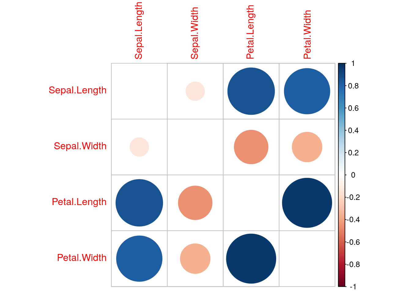
training.separate.cor=training.separate[,-highlyCor] #remove highly correlated predictors from training
testing.separate.cor=testing.separate[,-highlyCor] #remove highly correlated predictors from test
Here, we have one highly correlated variable, Petal Length.
Skewness
caret provides various methods for transforming skewed variables to normality, including the Box-Cox (Box and Cox 1964) and Yeo-Johnson (Yeo and Johnson 2000) transformations. Here we try using the Box-Cox method.
#perform boxcox scaling on each predictor
training.separate.boxcox=training.separate
training.separate.boxcox$Sepal.Length=predict(BoxCoxTrans(iris$Sepal.Length),
                                       training.separate.cor$Sepal.Length)
training.separate.boxcox$Sepal.Width=predict(BoxCoxTrans(iris$Sepal.Width),
                                      training.separate.cor$Sepal.Width)
training.separate.boxcox$Petal.Width=predict(BoxCoxTrans(iris$Petal.Width),
                                      training.separate.cor$Petal.Width)

testing.separate.boxcox=testing.separate
testing.separate.boxcox$Sepal.Length=predict(BoxCoxTrans(iris$Sepal.Length),
                                      testing.separate.cor$Sepal.Length)
testing.separate.boxcox$Sepal.Width=predict(BoxCoxTrans(iris$Sepal.Width),
                                     testing.separate.cor$Sepal.Width)
testing.separate.boxcox$Petal.Width=predict(BoxCoxTrans(iris$Petal.Width),
                                     testing.separate.cor$Petal.Width)

summary(training.separate.boxcox)
## Sepal.Length Sepal.Width Petal.Length Petal.Width
## Min. :1.459 Min. :0.7705 Min. :1.100 Min. :-1.24802
## 1st Qu.:1.629 1st Qu.:1.2064 1st Qu.:1.600 1st Qu.:-0.85734
## Median :1.758 Median :1.3013 Median :4.200 Median : 0.28414
## Mean :1.755 Mean :1.3167 Mean :3.747 Mean : 0.06693
## 3rd Qu.:1.856 3rd Qu.:1.4357 3rd Qu.:5.100 3rd Qu.: 0.70477
## Max. :2.041 Max. :1.8656 Max. :6.900 Max. : 1.22144
## Species
## setosa :35
## versicolor:35
## virginica :35
##
##
## summary(testing.separate.boxcox)## Sepal.Length Sepal.Width Petal.Length Petal.Width
## Min. :1.504 Min. :0.9462 Min. :1.000 Min. :-1.24802
## 1st Qu.:1.629 1st Qu.:1.2064 1st Qu.:1.500 1st Qu.:-0.85734
## Median :1.740 Median :1.3013 Median :4.500 Median : 0.28414
## Mean :1.756 Mean :1.3206 Mean :3.784 Mean : 0.08104
## 3rd Qu.:1.841 3rd Qu.:1.4357 3rd Qu.:5.100 3rd Qu.: 0.70477
## Max. :2.067 Max. :1.7566 Max. :6.700 Max. : 1.15156
## Species
## setosa :15
## versicolor:15
## virginica :15
##
##
## In this situation it is also important to centre and scale each predictor. A predictor variable is centered by subtracting the mean of the predictor from each value. To scale a predictor variable, each value is divided by its standard deviation. After centring and scaling the predictor variable has a mean of 0 and a standard deviation of 1.
2.4.1.2 Using preProcess function
Instead of using separate functions, we can add all the preprocessing into one function call to preProcess.
#The options for preprocessing are "BoxCox", "YeoJohnson", "expoTrans", "center", "scale", "range", "knnImpute", "bagImpute", "medianImpute", "pca", "ica", "spatialSign", "corr", "zv", "nzv", and "conditionalX"
calculatePreProcess <- preProcess(training,
                                  method = c("center", "scale","corr","nzv","BoxCox")) #perform preprocessing
calculatePreProcess
## Created from 105 samples and 5 variables
##
## Pre-processing:
## - Box-Cox transformation (3)
## - centered (3)
## - ignored (1)
## - removed (1)
## - scaled (3)
##
## Lambda estimates for Box-Cox transformation:
## 0.2, 0.5, 0.6training.preprocess <- predict(calculatePreProcess, training) #apply preprocessing to training data
summary(training.preprocess)## Sepal.Length Sepal.Width Petal.Width Species
## Min. :-2.073067 Min. :-2.56222 Min. :-1.6440 setosa :35
## 1st Qu.:-0.902243 1st Qu.:-0.54615 1st Qu.:-1.1556 versicolor:35
## Median : 0.007114 Median :-0.08917 Median : 0.2716 virginica :35
## Mean : 0.000000 Mean : 0.00000 Mean : 0.0000
## 3rd Qu.: 0.719086 3rd Qu.: 0.56862 3rd Qu.: 0.7974
## Max. : 2.095041 Max. : 2.75526 Max. : 1.4434#Petal.Length is removed
testing.preprocess <- predict(calculatePreProcess, testing) #apply same preprocessing to testing data
summary(testing.preprocess)## Sepal.Length Sepal.Width Petal.Width Species
## Min. :-1.76500 Min. :-1.76576 Min. :-1.64398 setosa :15
## 1st Qu.:-0.90224 1st Qu.:-0.54615 1st Qu.:-1.15555 versicolor:15
## Median :-0.11722 Median :-0.08917 Median : 0.27156 virginica :15
## Mean : 0.01216 Mean : 0.01591 Mean : 0.01764
## 3rd Qu.: 0.60424 3rd Qu.: 0.56862 3rd Qu.: 0.79745
## Max. : 2.28989 Max. : 2.18903 Max. : 1.35603dtreeIris.preprocess <- train(
Species ~ .,
data = training.preprocess,
method = "rpart" #this is a decision tree but we will get to more information about that later
)
dtreeIris.preprocess## CART
##
## 105 samples
## 3 predictor
## 3 classes: 'setosa', 'versicolor', 'virginica'
##
## No pre-processing
## Resampling: Bootstrapped (25 reps)
## Summary of sample sizes: 105, 105, 105, 105, 105, 105, ...
## Resampling results across tuning parameters:
##
## cp Accuracy Kappa
## 0.0000000 0.9292922 0.8922829
## 0.4142857 0.7305999 0.6121617
## 0.5000000 0.4787046 0.2760704
##
## Accuracy was used to select the optimal model using the largest value.
## The final value used for the model was cp = 0.2.4.2 Training different types of models
One of the primary tools in the package is this train function which can be used to evaluate, using resampling, the effect of model tuning parameters on performance, choose the ‘optimal’ model across these parameters and estimate model performance from a training set.
caret enables the easy use of many different types of models, a few of which we will cover in the course. The full list is here https://topepo.github.io/caret/available-models.html
We can change the model we use by changing the ‘method’ parameter in the train function. For example:
#decision tree
dtreeIris <- train(
    Species ~ .,
    data = training.preprocess, ##make sure you use the preprocessed version
    method = "rpart" #specifies decision tree
)

#support vector machine
svmIris <- train(
    Species ~ .,
    data = training.preprocess, ##make sure you use the preprocessed version
    method = "svmLinear" #specifies support vector machine with linear kernel
)

#random forest
randomForestIris <- train(
    Species ~ .,
    data = training.preprocess, ##make sure you use the preprocessed version
    method = "rf" ##specifies random forest
)
## note: only 2 unique complexity parameters in default grid. Truncating the grid to 2 .2.4.2.1 Adding preprocessing within training
We can combine the preprocessing step with training the model, using the preProc parameter in caret’s train function.
dtreeIris <- train(
    Species ~ ., ## this means the model should classify Species using the other features
    data = training, ## specifies training data (without preprocessing)
    method = "rpart", ## uses decision tree
    preProc = c("center", "scale","nzv","corr","BoxCox") ##this performs the preprocessing within model training
)
dtreeIris
## CART
##
## 105 samples
## 4 predictor
## 3 classes: 'setosa', 'versicolor', 'virginica'
##
## Pre-processing: centered (3), scaled (3), Box-Cox transformation (3), remove (1)
## Resampling: Bootstrapped (25 reps)
## Summary of sample sizes: 105, 105, 105, 105, 105, 105, ...
## Resampling results across tuning parameters:
##
## cp Accuracy Kappa
## 0.0000000 0.9191387 0.8770505
## 0.4285714 0.7166744 0.5883769
## 0.5000000 0.5276405 0.3239631
##
## Accuracy was used to select the optimal model using the largest value.
## The final value used for the model was cp = 0.2.4.3 Cross-validation
As we talked about in the last session, cross-validation is important to ensure the robustness of our models. We can specify how we want to perform cross-validation to caret.
train_ctrl = trainControl(method='cv',
                          number=10) #10-fold cross-validation

dtreeIris.10fold <- train(
    Species ~ .,
    data = training,
    method = "rpart",
    preProc = c("center", "scale","nzv","corr","BoxCox"),
    trControl = train_ctrl #train decision tree with 10-fold cross-validation
)
dtreeIris.10fold
## CART
##
## 105 samples
## 4 predictor
## 3 classes: 'setosa', 'versicolor', 'virginica'
##
## Pre-processing: centered (3), scaled (3), Box-Cox transformation (3), remove (1)
## Resampling: Cross-Validated (10 fold)
## Summary of sample sizes: 94, 95, 94, 95, 94, 94, ...
## Resampling results across tuning parameters:
##
## cp Accuracy Kappa
## 0.0000000 0.9336364 0.8997500
## 0.4285714 0.6563636 0.4960712
## 0.5000000 0.3763636 0.1285714
##
## Accuracy was used to select the optimal model using the largest value.
## The final value used for the model was cp = 0.You may notice that every time you run the last chunk you get slightly different answers. To make our analysis reproducible, we need to set some seeds. Rather than setting a single seed, we need to set quite a few as caret uses them in different places.
set.seed(42)
seeds = vector(mode='list',length=11) #this is #folds+1 so 10+1
for (i in 1:10) seeds[[i]] = sample.int(1000,10)
seeds[[11]] = sample.int(1000,1)

train_ctrl_seed = trainControl(method='cv',
                          number=10,
                          seeds=seeds) #use our seeds in the cross-validation


dtreeIris.10fold.seed <- train(
    Species ~ .,
    data = training,
    method = "rpart",
    preProc = c("center", "scale","nzv","corr","BoxCox"),
    trControl = train_ctrl_seed
)
dtreeIris.10fold.seed
## CART
##
## 105 samples
## 4 predictor
## 3 classes: 'setosa', 'versicolor', 'virginica'
##
## Pre-processing: centered (3), scaled (3), Box-Cox transformation (3), remove (1)
## Resampling: Cross-Validated (10 fold)
## Summary of sample sizes: 94, 94, 95, 95, 94, 95, ...
## Resampling results across tuning parameters:
##
## cp Accuracy Kappa
## 0.0000000 0.9134848 0.8703217
## 0.4285714 0.6375758 0.4707576
## 0.5000000 0.4151515 0.1714286
##
## Accuracy was used to select the optimal model using the largest value.
## The final value used for the model was cp = 0.If you try running this chunk multiple times, you will see the same answer each time
If you wanted to use repeated cross-validation instead of cross-validation, you can use:
set.seed(42)
seeds = vector(mode='list',length=101) #you need length #folds*#repeats + 1 so 10*10 + 1 here
for (i in 1:100) seeds[[i]] = sample.int(1000,10)
seeds[[101]] = sample.int(1000,1)

train_ctrl_seed_repeated = trainControl(method='repeatedcv',
                              number=10, #number of folds
                              repeats=10, #number of times to repeat cross-validation
                              seeds=seeds)


dtreeIris.10fold.seed.repeated <- train(
    Species ~ .,
    data = training,
    method = "rpart",
    preProc = c("center", "scale","nzv","corr","BoxCox"),
    trControl = train_ctrl_seed_repeated
)
dtreeIris.10fold.seed.repeated
## CART
##
## 105 samples
## 4 predictor
## 3 classes: 'setosa', 'versicolor', 'virginica'
##
## Pre-processing: centered (3), scaled (3), Box-Cox transformation (3), remove (1)
## Resampling: Cross-Validated (10 fold, repeated 10 times)
## Summary of sample sizes: 94, 95, 94, 93, 95, 95, ...
## Resampling results across tuning parameters:
##
## cp Accuracy Kappa
## 0.0000000 0.9355000 0.90268112
## 0.4285714 0.6628788 0.50378893
## 0.5000000 0.3666970 0.09857143
##
## Accuracy was used to select the optimal model using the largest value.
## The final value used for the model was cp = 0.2.4.4 Optimising hyperparameters
For different models, we need optimise different hyperparameters. To specify the different values we wish to consider, we use the tuneGrid or tuneLength parameters. In the decision tree example, we can optimise the cp value. Instead of looking at only 3 values, we may want to look at 10:
dtreeIris.hyperparam <- train(
    Species ~ .,
    data = training,
    method = "rpart",
    preProc = c("center", "scale","nzv","corr","BoxCox"),
    trControl = train_ctrl_seed_repeated,
    tuneLength = 10 #pick number of different hyperparam values to try
)
dtreeIris.hyperparam
## CART
##
## 105 samples
## 4 predictor
## 3 classes: 'setosa', 'versicolor', 'virginica'
##
## Pre-processing: centered (3), scaled (3), Box-Cox transformation (3), remove (1)
## Resampling: Cross-Validated (10 fold, repeated 10 times)
## Summary of sample sizes: 95, 94, 95, 94, 94, 95, ...
## Resampling results across tuning parameters:
##
## cp Accuracy Kappa
## 0.00000000 0.9314899 0.8961806
## 0.05555556 0.9314899 0.8961806
## 0.11111111 0.9314899 0.8961806
## 0.16666667 0.9314899 0.8961806
## 0.22222222 0.9314899 0.8961806
## 0.27777778 0.9314899 0.8961806
## 0.33333333 0.9314899 0.8961806
## 0.38888889 0.9314899 0.8961806
## 0.44444444 0.6409091 0.4737835
## 0.50000000 0.3718182 0.1071429
##
## Accuracy was used to select the optimal model using the largest value.
## The final value used for the model was cp = 0.3888889.We will see more example of this parameter as we explore different types of models.
2.4.5 Using dummy variables with the Sacramento dataset
If you have categorical predictors instead of continuous numeric variables, you may need to convert your categorical variable to a series of dummy variables. We will show this method on the Sacramento dataset.
From the documentation: This data frame contains house and sale price data for 932 homes in Sacramento CA. The original data were obtained from the website for the SpatialKey software. From their website: “The Sacramento real estate transactions file is a list of 985 real estate transactions in the Sacramento area reported over a five-day period, as reported by the Sacramento Bee.” Google was used to fill in missing/incorrect data.
data("Sacramento") ##loads the dataset, which can be accessed under the variable name Sacramento
?Sacramento
str(Sacramento)
## 'data.frame': 932 obs. of 9 variables:
## $ city : Factor w/ 37 levels "ANTELOPE","AUBURN",..: 34 34 34 34 34 34 34 34 29 31 ...
## $ zip : Factor w/ 68 levels "z95603","z95608",..: 64 52 44 44 53 65 66 49 24 25 ...
## $ beds : int 2 3 2 2 2 3 3 3 2 3 ...
## $ baths : num 1 1 1 1 1 1 2 1 2 2 ...
## $ sqft : int 836 1167 796 852 797 1122 1104 1177 941 1146 ...
## $ type : Factor w/ 3 levels "Condo","Multi_Family",..: 3 3 3 3 3 1 3 3 1 3 ...
## $ price : int 59222 68212 68880 69307 81900 89921 90895 91002 94905 98937 ...
## $ latitude : num 38.6 38.5 38.6 38.6 38.5 ...
## $ longitude: num -121 -121 -121 -121 -121 ...dummies = dummyVars(price ~ ., data = Sacramento) #convert the categorical variables to dummies
Sacramento.dummies = data.frame(predict(dummies, newdata = Sacramento))
Sacramento.dummies$price=Sacramento$priceOnce we have dummified, we can just split the data into training and test and train a model like with the Iris data.
set.seed(23)
trainTestPartition.Sacramento<-createDataPartition(y=Sacramento.dummies$price, #the class label, caret ensures an even split of classes
                                        p=0.7, #proportion of samples assigned to train
                                        list=FALSE)
training.Sacramento <- Sacramento.dummies[ trainTestPartition.Sacramento,]
testing.Sacramento  <- Sacramento.dummies[-trainTestPartition.Sacramento,]
lmSacramento <- train(
price ~ .,
data = training.Sacramento,
method = "lm",
preProc = c("center", "scale","nzv","corr","BoxCox")
)
lmSacramento## Linear Regression
##
## 655 samples
## 113 predictors
##
## Pre-processing: centered (10), scaled (10), Box-Cox transformation (4),
## remove (103)
## Resampling: Bootstrapped (25 reps)
## Summary of sample sizes: 655, 655, 655, 655, 655, 655, ...
## Resampling results:
##
## RMSE Rsquared MAE
## 87078.53 0.5843419 62112.79
##
## Tuning parameter 'intercept' was held constant at a value of TRUEWe can also train without using dummy variables and compare.
training.Sacramento.nondummy <- Sacramento[ trainTestPartition.Sacramento,]
testing.Sacramento.nondummy  <- Sacramento[-trainTestPartition.Sacramento,]

lmSacramento.nondummy <- train(
    price ~ .,
    data = training.Sacramento.nondummy,
    method = "lm",
    preProc = c("center", "scale","nzv","corr","BoxCox")
)
lmSacramento.nondummy
## Linear Regression
##
## 655 samples
## 8 predictor
##
## Pre-processing: centered (10), scaled (10), Box-Cox transformation (4),
## remove (100)
## Resampling: Bootstrapped (25 reps)
## Summary of sample sizes: 655, 655, 655, 655, 655, 655, ...
## Resampling results:
##
## RMSE Rsquared MAE
## 86605.34 0.5832732 61987.72
##
## Tuning parameter 'intercept' was held constant at a value of TRUE