13  Correlations

Learning outcomes

Questions

• What are correlation coefficients?
• What kind of correlation coefficients are there and when do I use them?

Objectives

• Be able to calculate correlation coefficients in R or Python
• Use visual tools to explore correlations between variables
• Know the limitations of correlation coefficients

13.1 Libraries and functions

Click to expand

R

13.1.1 Libraries

# A collection of R packages designed for data science
library(tidyverse)

13.1.2 Functions

# Computes the absolute value
base::abs()

# Creates a matrix of scatter plots
graphics::pairs()

# Computes a correlation matrix
stats::cor()

# Creates a heat map
stats::heatmap()

# Turns object into tibble
tibble::as.tibble()

# Lengthens the data
tidyr::pivot_longer()

Python

13.1.3 Libraries

# A Python data analysis and manipulation tool
import pandas as pd

# Python equivalent of `ggplot2`
from plotnine import *

13.1.4 Functions

# Compute pairwise correlation of columns
pandas.DataFrame.corr()

# Plots the first few rows of a DataFrame
pandas.DataFrame.head()

# Query the columns of a DataFrame with a boolean expression
pandas.DataFrame.query()

# Set the name of the axis for the index or columns
pandas.DataFrame.rename_axis()

# Unpivot a DataFrame from wide to long format
pandas.melt()

# Reads in a .csv file
pandas.read_csv()

13.2 Purpose and aim

Correlation refers to the relationship of two variables (or data sets) to one another. Two data sets are said to be correlated if they are not independent from one another. Correlations can be useful because they can indicate if a predictive relationship may exist. However just because two data sets are correlated does not mean that they are causally related.

13.3 Data and hypotheses

We will use the USArrests data set for this example. This rather bleak data set contains statistics in arrests per 100,000 residents for assault, murder and robbery in each of the 50 US states in 1973, alongside the proportion of the population who lived in urban areas at that time. USArrests is a data frame with 50 observations of five variables: state, murder, assault, urban_pop and robbery.

We will be using these data to explore if there are correlations between these variables.

The data are stored in the file data/CS3-usarrests.csv.

13.4 Summarise and visualise

First, we load the data:

R

# load the data
USArrests <- read_csv("data/CS3-usarrests.csv")

# have a look at the data
USArrests

# A tibble: 50 × 5
   state       murder assault urban_pop robbery
   <chr>        <dbl>   <dbl>     <dbl>   <dbl>
 1 Alabama       13.2     236        58    21.2
 2 Alaska        10       263        48    44.5
 3 Arizona        8.1     294        80    31  
 4 Arkansas       8.8     190        50    19.5
 5 California     9       276        91    40.6
 6 Colorado       7.9     204        78    38.7
 7 Connecticut    3.3     110        77    11.1
 8 Delaware       5.9     238        72    15.8
 9 Florida       15.4     335        80    31.9
10 Georgia       17.4     211        60    25.8
# ℹ 40 more rows

We can create a visual overview of the potential correlations that might exist between the variables. There are different ways of doing this, for example by creating scatter plots between variable pairs:

# murder vs robbery
ggplot(USArrests,
       aes(x = murder, y = robbery)) +
    geom_point()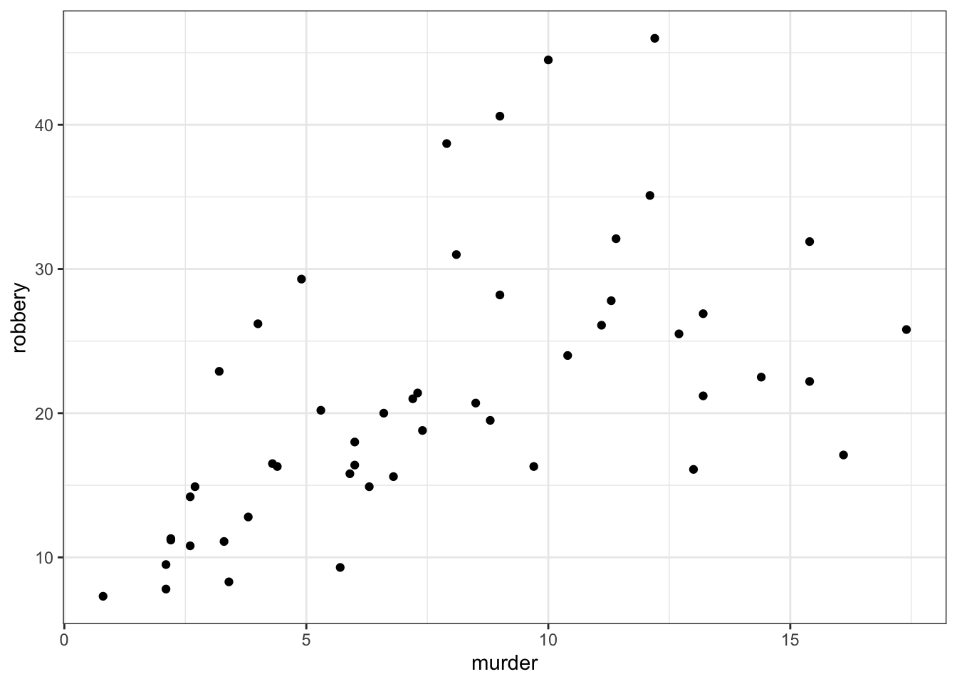

# assault vs urban_pop
ggplot(USArrests,
       aes(x = assault, y = urban_pop)) +
    geom_point()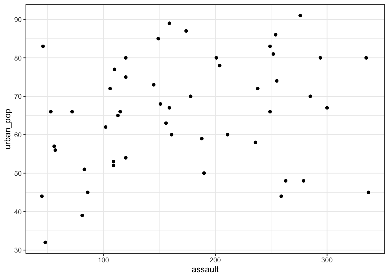

This gets a bit tedious if there are many unique variable pairs. Unfortunately ggplot() does not have a pairwise function, but we can borrow the one from base R. The pairs() function only wants numerical data, so we need to remove the state column for this. The pairs() function has a lower.panel argument that allows you to remove duplicate combinations (after all murder vs assault is the same as assault vs murder):

USArrests %>% 
    select(-state) %>% 
    pairs(lower.panel = NULL)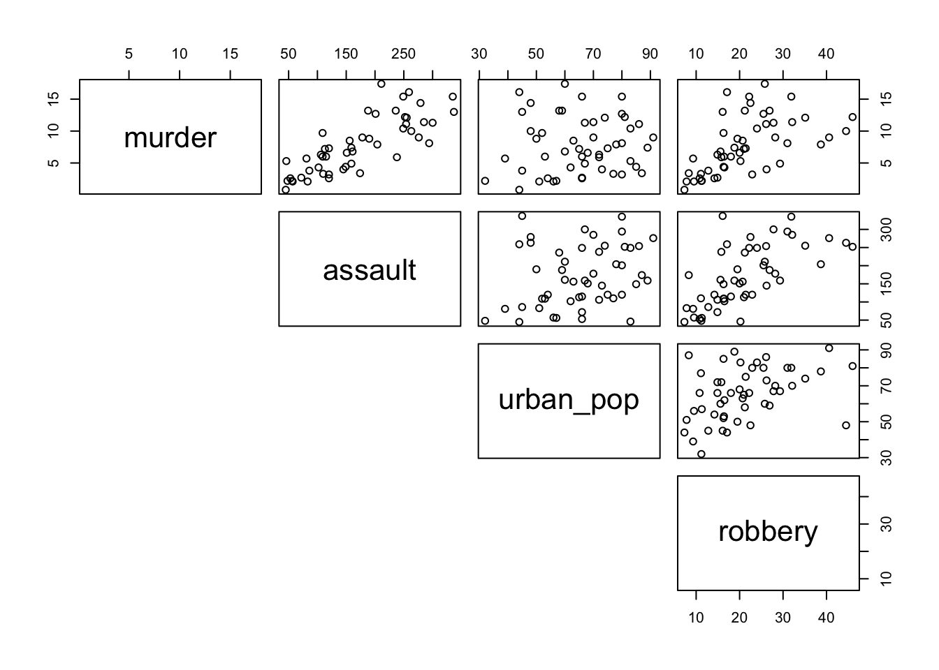

Python

First, we load the data:

USArrests_py = pd.read_csv("data/CS3-usarrests.csv")

USArrests_py.head()

        state  murder  assault  urban_pop  robbery
0     Alabama    13.2      236         58     21.2
1      Alaska    10.0      263         48     44.5
2     Arizona     8.1      294         80     31.0
3    Arkansas     8.8      190         50     19.5
4  California     9.0      276         91     40.6

We can create a visual overview of the potential correlations that might exist between the variables. There are different ways of doing this, for example by creating scatter plots between variable pairs:

# murder vs robbery
(ggplot(USArrests_py,
       aes(x = "murder",
           y = "robbery")) +
     geom_point())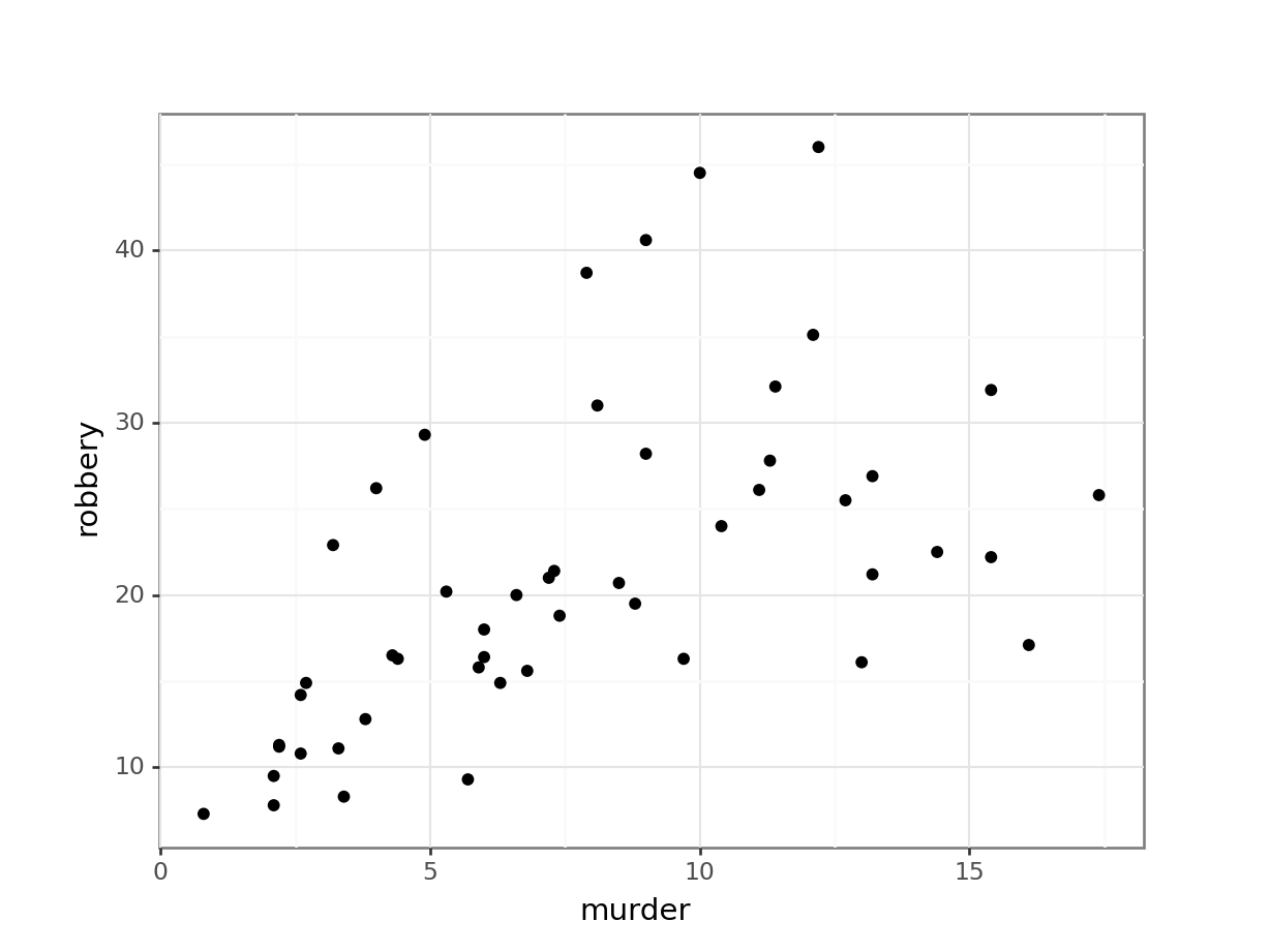

# assault vs urban_pop
(ggplot(USArrests_py,
       aes(x = "assault",
           y = "urban_pop")) +
     geom_point())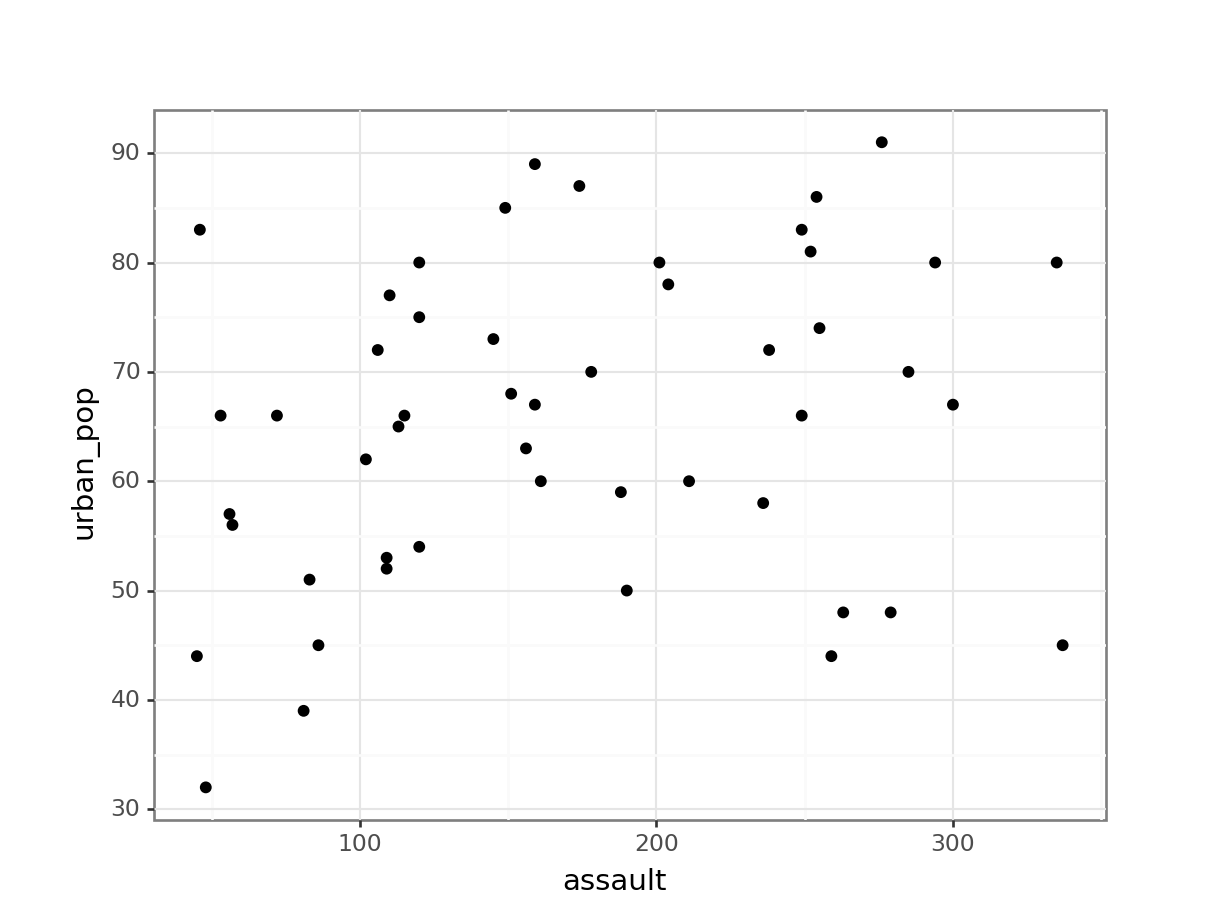

This gets a bit tedious if there are many unique variable pairs. There is an option to automatically create a matrix of scatter plots, using Seaborn. But that would involve installing the seaborn package just for this. And frankly, I don’t want to - not least because staring at tons of scatter plots is probably not the best way forward anyway!

If you have your heart set on creating a pairplot, then have a look at the seaborn documentation.

From the visual inspection we can see that there appears to be a slight positive correlation between all pairs of variables, although this may be very weak in some cases (murder and urban_pop for example).

13.5 Correlation coefficients

Instead of visualising the variables against each other in a scatter plot, we can also calculate correlation coefficients for each variable pair. There are different types of correlation coefficients, but the most well-known one is probably Pearson’s r. This is a measure of the linear correlation between two variables. It has a value between -1 and +1, where +1 means a perfect positive correlation, -1 means a perfect negative correlation and 0 means no correlation at all.

There are other correlation coefficients, most notably the Spearman’s rank correlation coefficient, a non-parametric measure of rank correlation and is generally less sensitive to outliers.

So, let’s calculate Pearson’s r for our data:

R

We can do this using the cor() function. Since we can only calculate correlations between numbers, we have to remove the state column from our data before calculating the correlations:

USArrests %>% 
    select(-state) %>% 
    cor()

              murder   assault  urban_pop   robbery
murder    1.00000000 0.8018733 0.06957262 0.5635788
assault   0.80187331 1.0000000 0.25887170 0.6652412
urban_pop 0.06957262 0.2588717 1.00000000 0.4113412
robbery   0.56357883 0.6652412 0.41134124 1.0000000

This gives us a numerical overview of the Pearson’s r correlation coefficients between each variable pair. Note that across the diagonal the correlation coefficients are 1 - this should make sense since, for example, murder is perfectly correlated with itself.

As before, the values are mirrored across the diagonal, since the correlation between, for example, murder and assault is the same as the one between assault and murder.

13.5.1 Visualise the correlation matrix

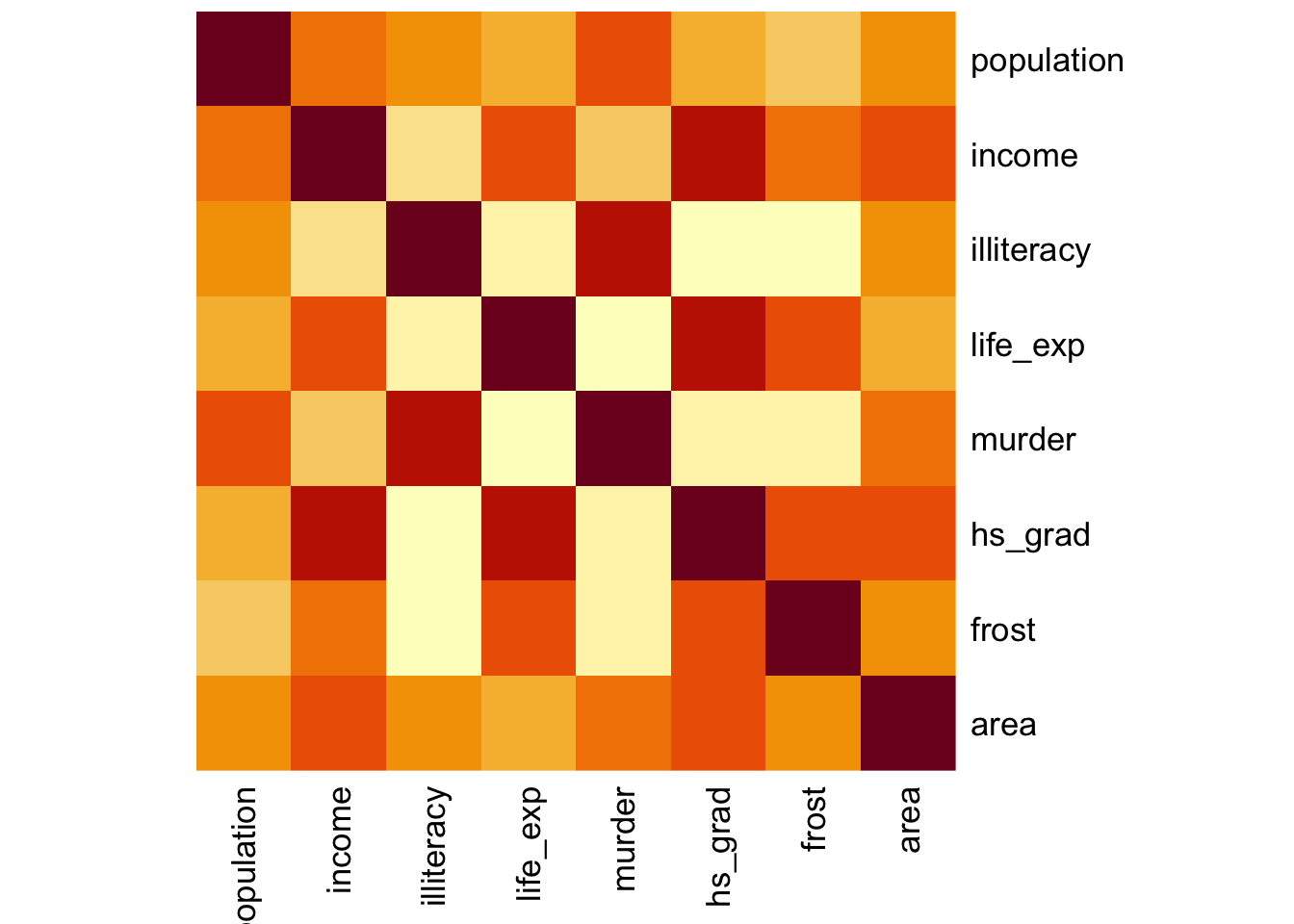
Just staring at a matrix of numbers might not be very useful. It would be good to create some sort of heatmap of the values, so we can visually inspect the data a bit better. There are dedicated packages that allow you to do this (for example the corrr) package).

Here we’ll just use the standard stats::heatmap() function. The symm argument tells the function that we have a symmetric matrix and in conjunction with the Rowv = NA argument stops the plot from reordering the rows and columns. The Rowv = NA argument also stops the function from adding dendrograms to the margins of the plot.

The plot itself is coloured from yellow, indicating the smallest values (which in this case correspond to no difference in correlation coefficients), through orange to dark red, indicating the biggest values (which in this case correspond to the variables with the biggest difference in correlation coefficients).

The plot is symmetric along the leading diagonal (hopefully for obvious reasons).

USArrests %>% 
  select(-state) %>% 
  cor() %>% 
  heatmap(symm = TRUE, Rowv = NA)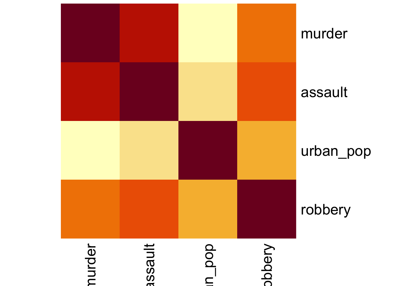

Alternative method 1: ggplot

Before we can plot the data we need to reformat the data. We’re taking the following steps:

1. we calculate the correlation matrix with cor() using the (default) method of method = "pearson"
2. convert the output to a tibble so we can use
3. pivot_longer() to reformat the data into pairwise variables and a column with the Pearson’s r value
4. use the mutate() and round() functions to round the Pearson’s r values

USArrests_pear <- USArrests %>% 
    select(-state) %>% 
    cor(method = "pearson") %>% 
    as_tibble(rownames = "var1") %>% 
    pivot_longer(cols = -var1,
                 names_to = "var2",
                 values_to = "pearson_cor") %>% 
    mutate(pearson_cor = round(pearson_cor, digits = 3))

The output of that looks like this:

head(USArrests_pear)

# A tibble: 6 × 3
  var1    var2      pearson_cor
  <chr>   <chr>           <dbl>
1 murder  murder          1    
2 murder  assault         0.802
3 murder  urban_pop       0.07 
4 murder  robbery         0.564
5 assault murder          0.802
6 assault assault         1    

After all that, we can visualise the data with geom_tile(), adding the Pearson’s r values as text labels:

ggplot(USArrests_pear,
       aes(x = var1, y = var2, fill = pearson_cor)) +
    geom_tile() +
    geom_text(aes(label = pearson_cor),
              color = "white",
              size = 4)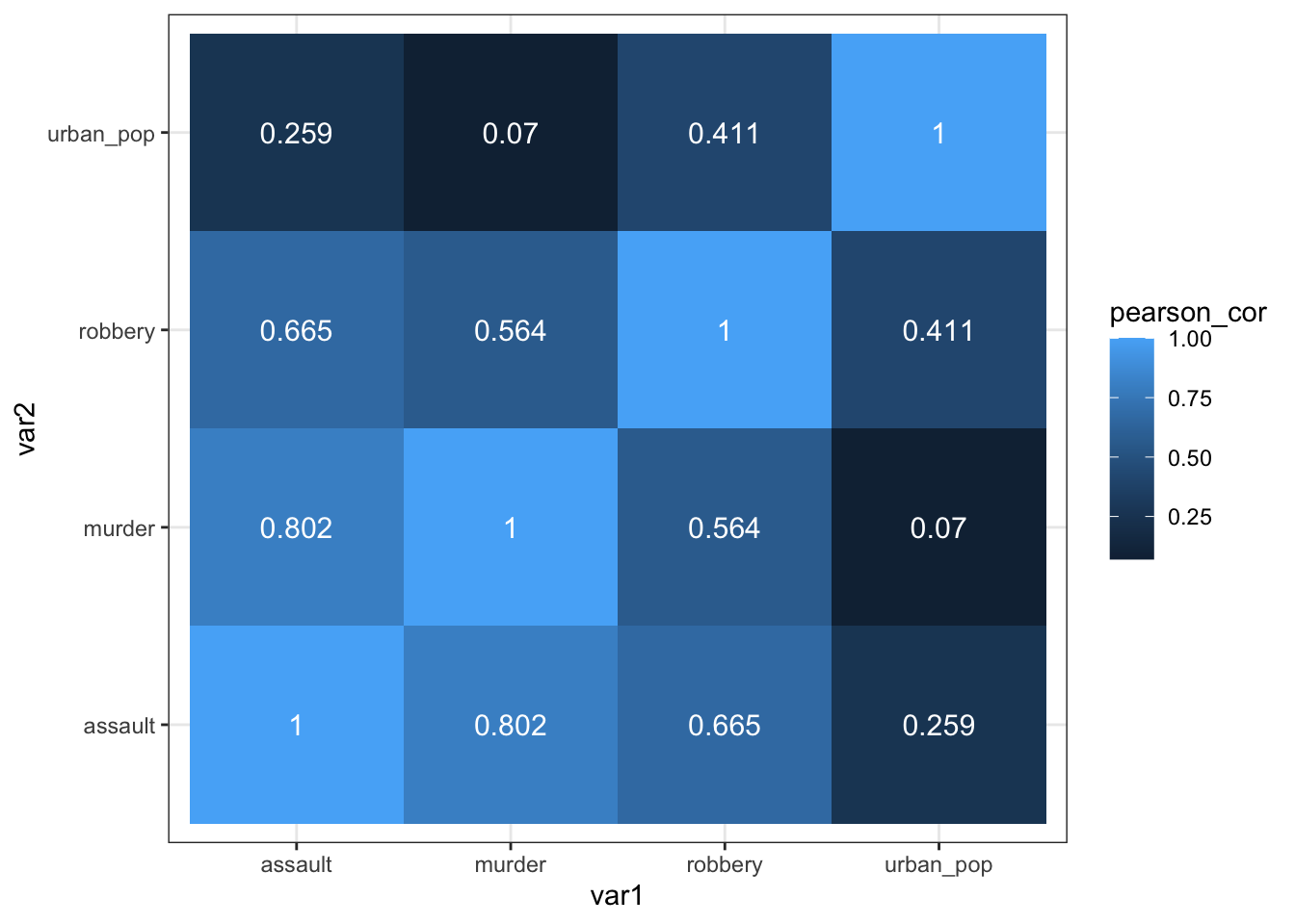

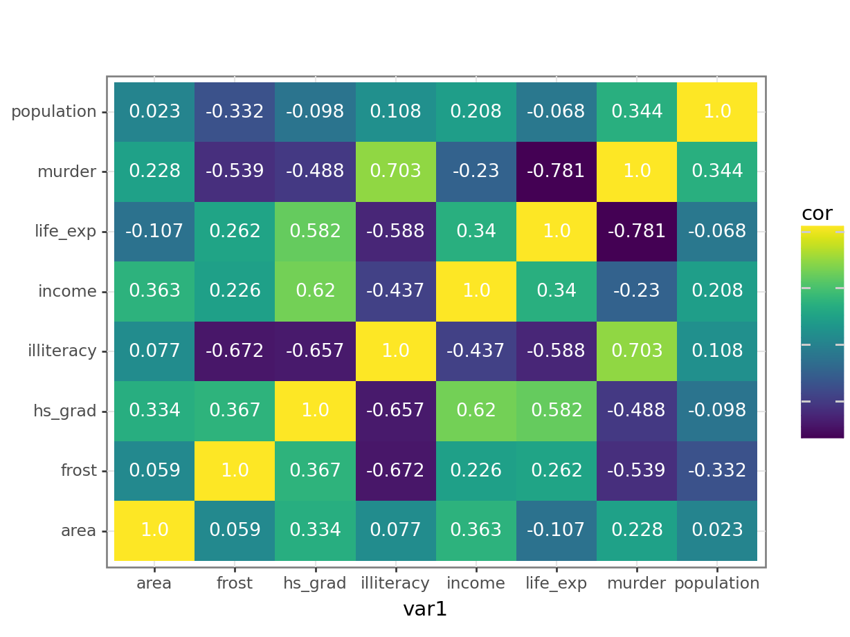
Alternative method 2: rstatix

As always, there are multiple ways to skin a proverbial cat. If you’d rather use a function from the rstatix package (which we’ve loaded before), then you can run the following code, which uses the rstatix::cor_test() function:

USArrests %>% 
    select(-state) %>% 
    cor_test() %>%
    select(var1, var2, cor) %>% 
    ggplot(aes(x = var1, y = var2, fill = cor)) +
    geom_tile() +
    geom_text(aes(label = cor),
              color = "white",
              size = 4)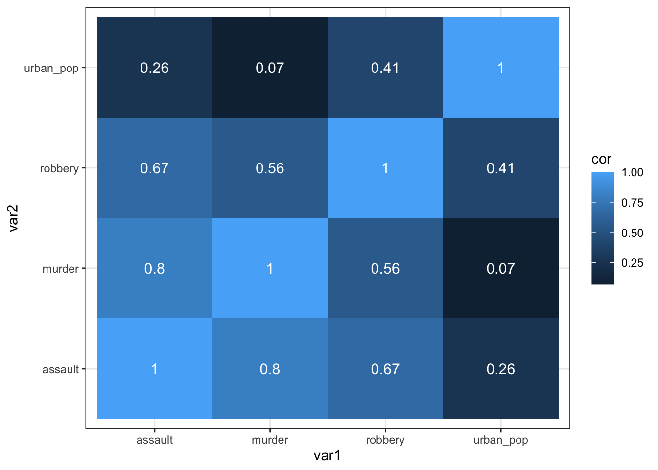

Python

We can do this using the pandas.DataFrame.corr() function. This function takes the default method = "pearson" and ignores any non-numerical columns (such as the state column in our data set).

USArrests_py.corr()

             murder   assault  urban_pop   robbery
murder     1.000000  0.801873   0.069573  0.563579
assault    0.801873  1.000000   0.258872  0.665241
urban_pop  0.069573  0.258872   1.000000  0.411341
robbery    0.563579  0.665241   0.411341  1.000000

This gives us a numerical overview of the Pearson’s r correlation coefficients between each variable pair. Note that across the diagonal the correlation coefficients are 1 - this should make sense since, for example, murder is perfectly correlated with itself.

As before, the values are mirrored across the diagonal, since the correlation between, for example, murder and assault is the same as the one between assault and murder.

13.5.2 Visualise the correlation matrix

Just staring at a matrix of numbers might not be very useful. It would be good to create some sort of heatmap of the values, so we can visually inspect the data a bit better.

# create correlation matrix
USArrests_cor_py = USArrests_py.corr()
# put the row names into a column
USArrests_cor_py = USArrests_cor_py.rename_axis("var1").reset_index()

USArrests_cor_py.head()

        var1    murder   assault  urban_pop   robbery
0     murder  1.000000  0.801873   0.069573  0.563579
1    assault  0.801873  1.000000   0.258872  0.665241
2  urban_pop  0.069573  0.258872   1.000000  0.411341
3    robbery  0.563579  0.665241   0.411341  1.000000

Now that we have the correlation matrix in a workable format, we need to restructure it so that we can plot the data. For this, we need to create a “long” format, using the melt() function.

USArrests_pear_py = pd.melt(USArrests_cor_py,
        id_vars=['var1'],
        value_vars=['murder', 'assault', 'urban_pop', 'robbery'],
        var_name='var2',
        value_name='cor').round(3)

Have a look at the structure:

USArrests_pear_py.head()

        var1     var2    cor
0     murder   murder  1.000
1    assault   murder  0.802
2  urban_pop   murder  0.070
3    robbery   murder  0.564
4     murder  assault  0.802

(ggplot(USArrests_pear_py,
        aes(x = "var1", y = "var2", fill = "cor")) +
     geom_tile() +
     geom_text(aes(label = "cor"),
               colour = "white",
               size = 10))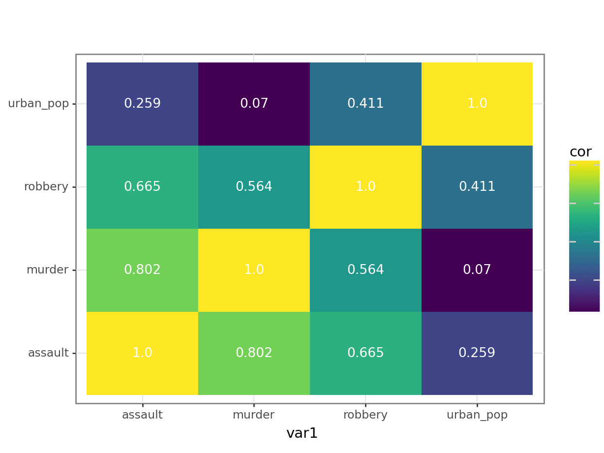

The correlation matrix and visualisations give us the insight that we need. The most correlated variables are murder and assault with an \(r\) value of 0.80. This appears to agree well with the set plots that we produced earlier.

13.6 Spearman’s rank correlation coefficient

This test first calculates the rank of the numerical data (i.e. their position from smallest (or most negative) to the largest (or most positive)) in the two variables and then calculates Pearson’s product moment correlation coefficient using the ranks. As a consequence, this test is less sensitive to outliers in the distribution.

R

USArrests %>% 
    select(-state) %>% 
    cor(method = "spearman")

             murder   assault urban_pop   robbery
murder    1.0000000 0.8172735 0.1067163 0.6794265
assault   0.8172735 1.0000000 0.2752133 0.7143681
urban_pop 0.1067163 0.2752133 1.0000000 0.4381068
robbery   0.6794265 0.7143681 0.4381068 1.0000000

Python

USArrests_py.corr(method = "spearman")

             murder   assault  urban_pop   robbery
murder     1.000000  0.817274   0.106716  0.679427
assault    0.817274  1.000000   0.275213  0.714368
urban_pop  0.106716  0.275213   1.000000  0.438107
robbery    0.679427  0.714368   0.438107  1.000000

13.7 Exercises

13.7.1 Pearson’s r

Exercise

Level:

Pearson’s correlation for USA state data

We will again use the data from the file data/CS3-statedata.csv data set for this exercise. The data set contains 50 rows and 8 columns, with column names: population, income, illiteracy, life_exp, murder, hs_grad, frost and area.

Visually identify 3 different pairs of variables that appear to be

1. the most positively correlated
2. the most negatively correlated
3. not correlated at all

Calculate Pearson’s r for all variable pairs and see how well you were able to identify correlation visually.

Answer

13.8 Answer

Visually determining the most negative/positively and uncorrelated pairs of variables:

R

USAstate <- read_csv("data/CS3-statedata.csv")

# have a look at the data
USAstate

# A tibble: 50 × 9
   state       population income illiteracy life_exp murder hs_grad frost   area
   <chr>            <dbl>  <dbl>      <dbl>    <dbl>  <dbl>   <dbl> <dbl>  <dbl>
 1 Alabama           3615   3624        2.1     69.0   15.1    41.3    20  50708
 2 Alaska             365   6315        1.5     69.3   11.3    66.7   152 566432
 3 Arizona           2212   4530        1.8     70.6    7.8    58.1    15 113417
 4 Arkansas          2110   3378        1.9     70.7   10.1    39.9    65  51945
 5 California       21198   5114        1.1     71.7   10.3    62.6    20 156361
 6 Colorado          2541   4884        0.7     72.1    6.8    63.9   166 103766
 7 Connecticut       3100   5348        1.1     72.5    3.1    56     139   4862
 8 Delaware           579   4809        0.9     70.1    6.2    54.6   103   1982
 9 Florida           8277   4815        1.3     70.7   10.7    52.6    11  54090
10 Georgia           4931   4091        2       68.5   13.9    40.6    60  58073
# ℹ 40 more rows

We basically repeat what we’ve done previously:

USAstate_pear <-USAstate %>% 
  select(-state) %>% 
  cor(method = "pearson")

Next, we can plot the data:

heatmap(USAstate_pear, symm = TRUE, Rowv = NA)

Python

First, we load the data:

USAstate_py = pd.read_csv("data/CS3-statedata.csv")

USAstate_py.head()

        state  population  income  illiteracy  ...  murder  hs_grad  frost    area
0     Alabama        3615    3624         2.1  ...    15.1     41.3     20   50708
1      Alaska         365    6315         1.5  ...    11.3     66.7    152  566432
2     Arizona        2212    4530         1.8  ...     7.8     58.1     15  113417
3    Arkansas        2110    3378         1.9  ...    10.1     39.9     65   51945
4  California       21198    5114         1.1  ...    10.3     62.6     20  156361

[5 rows x 9 columns]

# create correlation matrix
USAstate_cor_py = USAstate_py.corr()
# put the row names into a column
USAstate_cor_py = USAstate_cor_py.rename_axis("var1").reset_index()

USAstate_cor_py.head()

         var1  population    income  ...   hs_grad     frost      area
0  population    1.000000  0.208228  ... -0.098490 -0.332152  0.022544
1      income    0.208228  1.000000  ...  0.619932  0.226282  0.363315
2  illiteracy    0.107622 -0.437075  ... -0.657189 -0.671947  0.077261
3    life_exp   -0.068052  0.340255  ...  0.582216  0.262068 -0.107332
4      murder    0.343643 -0.230078  ... -0.487971 -0.538883  0.228390

[5 rows x 9 columns]

Now that we have the correlation matrix in a workable format, we need to restructure it so that we can plot the data. For this, we need to create a “long” format, using the melt() function. Note that we’re not setting the values_var argument. If not set, then it uses all but the id_vars column (which in our case is a good thing, since we don’t want to manually specify lots of column names).

USAstate_pear_py = pd.melt(USAstate_cor_py,
        id_vars=['var1'],
        var_name='var2',
        value_name='cor').round(3)

Have a look at the structure:

USArrests_pear_py.head()

        var1     var2    cor
0     murder   murder  1.000
1    assault   murder  0.802
2  urban_pop   murder  0.070
3    robbery   murder  0.564
4     murder  assault  0.802

(ggplot(USAstate_pear_py,
        aes(x = "var1", y = "var2", fill = "cor")) +
     geom_tile() +
     geom_text(aes(label = "cor"),
               colour = "white",
               size = 10))

It looks like:

1. illiteracy and murder are the most positively correlated pair
2. life_exp and murder are the most negatively correlated pair
3. population and area are the least correlated pair

We can explore that numerically, by doing the following:

R

First, we need to create the pairwise comparisons, with the relevant Pearson’s \(r\) values:

# build a contingency table with as.table()
# and create a dataframe with as.data.frame()
USAstate_pear_cont <- as.data.frame(as.table(USAstate_pear))
    
# and have a look
head(USAstate_pear_cont)

        Var1       Var2        Freq
1 population population  1.00000000
2     income population  0.20822756
3 illiteracy population  0.10762237
4   life_exp population -0.06805195
5     murder population  0.34364275
6    hs_grad population -0.09848975

Is this method obvious? No! Some creative Googling led to Stackoverflow and here we are. But, it does give us what we need.

Now that we have the paired comparisons, we can extract the relevant data:

# first we remove the same-pair correlations
USAstate_pear_cont <- USAstate_pear_cont %>% 
  filter(Freq != 1)

# most positively correlated pair
USAstate_pear_cont %>% 
  filter(Freq == max(Freq))

        Var1       Var2      Freq
1     murder illiteracy 0.7029752
2 illiteracy     murder 0.7029752

# most negatively correlated pair
USAstate_pear_cont %>% 
  filter(Freq == min(Freq))

      Var1     Var2       Freq
1   murder life_exp -0.7808458
2 life_exp   murder -0.7808458

# least correlated pair
USAstate_pear_cont %>% 
  filter(Freq == min(abs(Freq)))

        Var1       Var2       Freq
1       area population 0.02254384
2 population       area 0.02254384

Note that we use the minimum absolute value (with the abs() function) to find the least correlated pair.

Python

We take the correlation matrix in the long format:

USAstate_pear_py.head()

         var1        var2    cor
0  population  population  1.000
1      income  population  0.208
2  illiteracy  population  0.108
3    life_exp  population -0.068
4      murder  population  0.344

and use it to extract the relevant values:

# filter out self-pairs
df_cor = USAstate_pear_py.query("cor != 1")

# filter for the maximum correlation value
df_cor[df_cor.cor == df_cor.cor.max()]

          var1        var2    cor
20      murder  illiteracy  0.703
34  illiteracy      murder  0.703

# filter for the minimum correlation value
df_cor[df_cor.cor == df_cor.cor.min()]

        var1      var2    cor
28    murder  life_exp -0.781
35  life_exp    murder -0.781

# filter for the least correlated value
# create a column containing absolute values
df_cor["abs_cor"] = df_cor["cor"].abs()
df_cor[df_cor.abs_cor == df_cor.abs_cor.min()]

          var1        var2    cor  abs_cor
7         area  population  0.023    0.023
56  population        area  0.023    0.023

13.8.1 Spearman’s correlation

Exercise

Level:

Calculate Spearman’s correlation coefficient for the data/CS3-statedata.csv data set.

Which variable’s correlations are affected most by the use of the Spearman’s rank compared with Pearson’s r? Hint: think of a way to address this question programmatically.

Thinking about the variables, can you explain why this might this be?

Answer

13.9 Answer

In order to determine which variables are most affected by the choice of Spearman vs Pearson you could just plot both matrices out side by side and try to spot what was going on, but one of the reasons we’re using programming languages is that we can be a bit more programmatic about these things. Also, our eyes aren’t that good at processing and parsing this sort of information display. A better way would be to somehow visualise the data.

R

First, calculate the Pearson and Spearman correlation matrices (technically, we’ve done the Pearson one already, but we’re doing it again for clarity here).

cor_pear <- USAstate %>% 
    select(-state) %>% 
    cor(method = "pearson")

cor_spear <- USAstate %>% 
    select(-state) %>% 
    cor(method = "spearman")

We can calculate the difference between two matrices by subtracting them.

cor_diff <- cor_pear - cor_spear

Again, we could now just look at a grid of 64 numbers and see if we can spot the biggest differences, but our eyes aren’t that good at processing and parsing this sort of information display. A better way would be to visualise the data.

heatmap(abs(cor_diff), symm = TRUE, Rowv = NA)

The abs() function calculates the absolute value (i.e. just the magnitude) of the matrix values. This is just because I only care about situations where the two correlation coefficients are different from each other but I don’t care which is the larger. The symm argument tells the function that we have a symmetric matrix and in conjunction with the Rowv = NA argument stops the plot from reordering the rows and columns. The Rowv = NA argument also stops the function from adding dendrograms to the margins of the plot.

Python

First, calculate the Pearson and Spearman correlation matrices (technically, we’ve done the Pearson one already, but we’re doing it again for clarity here).

cor_pear_py = USAstate_py.corr(method = "pearson")
cor_spea_py = USAstate_py.corr(method = "spearman")

We can calculate the difference between two matrices by subtracting them.

cor_dif_py = cor_pear_py - cor_spea_py

Again, we could now just look at a grid of 64 numbers and see if we can spot the biggest differences, but our eyes aren’t that good at processing and parsing this sort of information display. A better way would be to visualise the data.

# get the row names in a column
cor_dif_py = cor_dif_py.rename_axis("var1").reset_index()

# reformat the data into a long format
# and round the values
cor_dif_py = pd.melt(cor_dif_py,
        id_vars=['var1'],
        var_name='var2',
        value_name='cor').round(3)
        
# create a column with absolute correlation difference values
cor_dif_py["abs_cor"] = cor_dif_py["cor"].abs()

# have a look at the final data frame
cor_dif_py.head()

         var1        var2    cor  abs_cor
0  population  population  0.000    0.000
1      income  population  0.084    0.084
2  illiteracy  population -0.205    0.205
3    life_exp  population  0.036    0.036
4      murder  population -0.002    0.002

Now we can plot the data:

(ggplot(cor_dif_py,
        aes(x = "var1", y = "var2", fill = "abs_cor")) +
     geom_tile() +
     geom_text(aes(label = "abs_cor"),
               colour = "white",
               size = 10))

All in all there is not a huge difference in correlation coefficients, since the values are all quite small. Most of the changes occur along the area variable. One possible explanation could be that certain states with a large area have a relatively large effect on the Pearson’s r coefficient. For example, Alaska has an area that is over twice as big as the next state - Texas.

If, for example, we’d look a bit closer then we would find for area and income that Pearson gives a value of 0.36, a slight positive correlation, whereas Spearman gives a value of 0.057, basically uncorrelated.

This means that this is basically ignored by Spearman.

Well done, Mr. Spearman.

13.10 Summary

Key points

• Correlation is the degree to which two variables are linearly related
• Correlation does not imply causation
• We can visualise correlations by plotting variables against each other or creating heatmap-type plots of the correlation coefficients
• Two main correlation coefficients are Pearson’s r and Spearman’s rank, with Spearman’s rank being less sensitive to outliers