12  Analysing count data

Learning outcomes

• Be able to identify count data
• Fit a Poisson regression model with count data
• Assess whether assumptions are met and test significance of the model

12.1 Context

We have now covered analysing binary responses and learned how to assess the quality and appropriateness of the resulting models. In the next sections we extend this further, by looking at a different type of response variable: count data. The humble count may look innocent, but often hides a whole lot of nuances that are hard to spot. So, pay attention!

12.2 Section setup

Click to expand

We’ll use the following libraries and data:

R

# Load required R libraries
library(tidyverse)
library(performance)

# Read in the required data
islands <- read_csv("data/islands.csv")
seatbelts <- read_csv("data/seatbelts.csv")

Python

# Load required Python libraries
import pandas as pd
import math
import statsmodels.api as sm
import statsmodels.formula.api as smf
from scipy.stats import *
from plotnine import *

# Read in the required data
islands = pd.read_csv("data/islands.csv")
seatbelts = pd.read_csv("data/seatbelts.csv")

The worked example in this chapter will use the islands dataset.

This is a dataset comprising 35 observations of two variables. For each small island in the dataset, the researcher recorded the number of unique species; they want to know if this can be predicted from the area (km²) of the island.

12.3 Load and visualise the data

First we load the data, then we visualise it.

R

islands <- read_csv("data/islands.csv")

head(islands)

# A tibble: 6 × 2
  species  area
    <dbl> <dbl>
1     114  12.1
2     130  13.4
3     113  13.7
4     109  14.5
5     118  16.8
6     136  19.0

Python

islands = pd.read_csv("data/islands.csv")

islands.head()

   species       area
0      114  12.076133
1      130  13.405439
2      113  13.723525
3      109  14.540359
4      118  16.792122

We can plot the data:

R

ggplot(islands, aes(x = area, y = species)) +
  geom_point()

Figure 12.1: Scatterplot of area and species

Python

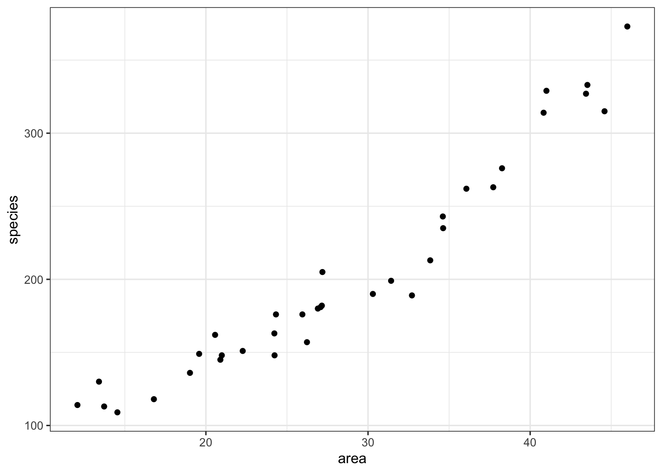
p = (ggplot(islands, aes(x = "area", y = "species")) +
   geom_point())

p.show()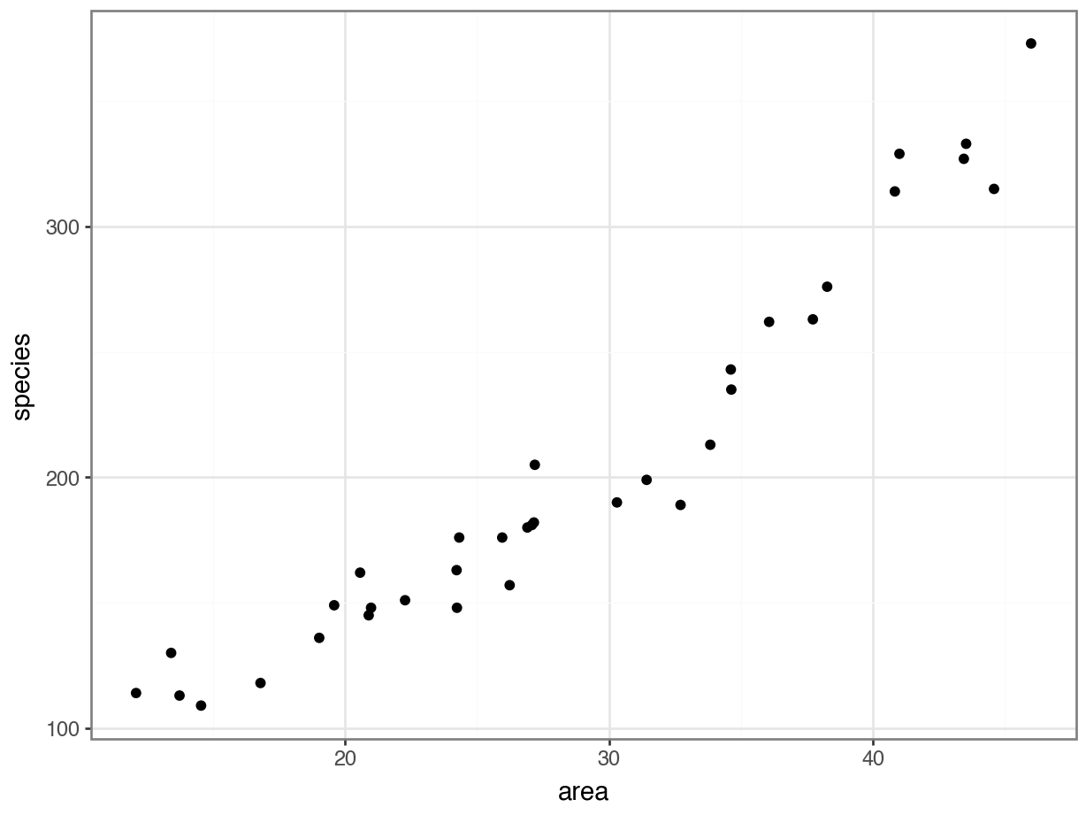

Figure 12.2: Scatterplot of area and species

Each dot on the scatterplot represents an island in the dataset.

It looks as though area definitely has some relationship with the number of species that we observe.

Next step is to try to model these data.

12.4 Constructing a model

The species variable is the outcome or response (since we’re interested in whether it’s predicted by area).

It qualifies as a count variable. It’s bounded at 0 and \(\infty\), and can only jump up in integers - in other words, you can’t have less than 0 species, or 6.3 species.

This means the best place to start is a Poisson regression. We fit these in a very similar way to a logistic regression, just with a different option specified for the family argument.

R

glm_isl <- glm(species ~ area,
               data = islands, family = "poisson")

and we look at the model summary:

summary(glm_isl)

Call:
glm(formula = species ~ area, family = "poisson", data = islands)

Coefficients:
            Estimate Std. Error z value Pr(>|z|)    
(Intercept) 4.241129   0.041322  102.64   <2e-16 ***
area        0.035613   0.001247   28.55   <2e-16 ***
---
Signif. codes:  0 '***' 0.001 '**' 0.01 '*' 0.05 '.' 0.1 ' ' 1

(Dispersion parameter for poisson family taken to be 1)

    Null deviance: 856.899  on 34  degrees of freedom
Residual deviance:  30.437  on 33  degrees of freedom
AIC: 282.66

Number of Fisher Scoring iterations: 3

The output is strikingly similar to the logistic regression models (who’d have guessed, eh?) and the main numbers to extract from the output are the coefficients (the two numbers underneath Estimate in the table above):

coefficients(glm_isl)

(Intercept)        area 
 4.24112904  0.03561346 

Python

model = smf.glm(formula = "species ~ area",
                family = sm.families.Poisson(),
                data = islands)

glm_isl = model.fit()

Let’s look at the model output:

print(glm_isl.summary())

                 Generalized Linear Model Regression Results                  
==============================================================================
Dep. Variable:                species   No. Observations:                   35
Model:                            GLM   Df Residuals:                       33
Model Family:                 Poisson   Df Model:                            1
Link Function:                    Log   Scale:                          1.0000
Method:                          IRLS   Log-Likelihood:                -139.33
Date:                Fri, 25 Jul 2025   Deviance:                       30.437
Time:                        08:28:46   Pearson chi2:                     30.3
No. Iterations:                     4   Pseudo R-squ. (CS):              1.000
Covariance Type:            nonrobust                                         
==============================================================================
                 coef    std err          z      P>|z|      [0.025      0.975]
------------------------------------------------------------------------------
Intercept      4.2411      0.041    102.636      0.000       4.160       4.322
area           0.0356      0.001     28.551      0.000       0.033       0.038
==============================================================================

The output is strikingly similar to the logistic regression models (who’d have guessed, eh?) and the main numbers to extract from the output are the coefficients (the two numbers underneath coef in the table above):

print(glm_isl.params)

Intercept    4.241129
area         0.035613
dtype: float64

12.4.1 The model equation

Now that we have the beta coefficients, we can place them inside an equation.

The left-hand side of this equation is the expected number of species, \(E(species)\).

On the right-hand side, we take the linear equation \(\beta_0 + \beta_1 * x_1\) and embed it inside the inverse link function, which in this case is just the exponential function.

It looks like this:

\[ E(species) = \exp(4.24 + 0.036 \times area) \]

Interpreting this requires a bit of thought (not much, but a bit).

The intercept coefficient, 4.24, is related to the number of species we would expect on an island of zero area. But in order to turn this number into something meaningful we have to exponentiate it.

Since \(\exp(4.24) \approx 69\), we can say that the baseline number of species the model expects on any island is 69.

The coefficient of area is the fun bit. For starters we can see that it is a positive number which does mean that increasing area leads to increasing numbers of species. Good so far.

But what does the value 0.036 actually mean? Well, if we exponentiate it as well, we get \(\exp(0.036) \approx 1.04\). This means that for every increase in area of 1 km² (the original units of the area variable), the number of species on the island is multiplied by 1.04.

So, an island of area km² will have \(1.04 \times 69 \approx 72\) species.

12.5 Plotting the Poisson regression

R

ggplot(islands, aes(area, species)) +
  geom_point() +
  geom_smooth(method = "glm", se = FALSE, fullrange = TRUE, 
              method.args = list(family = "poisson")) +
  xlim(10,50)

`geom_smooth()` using formula = 'y ~ x'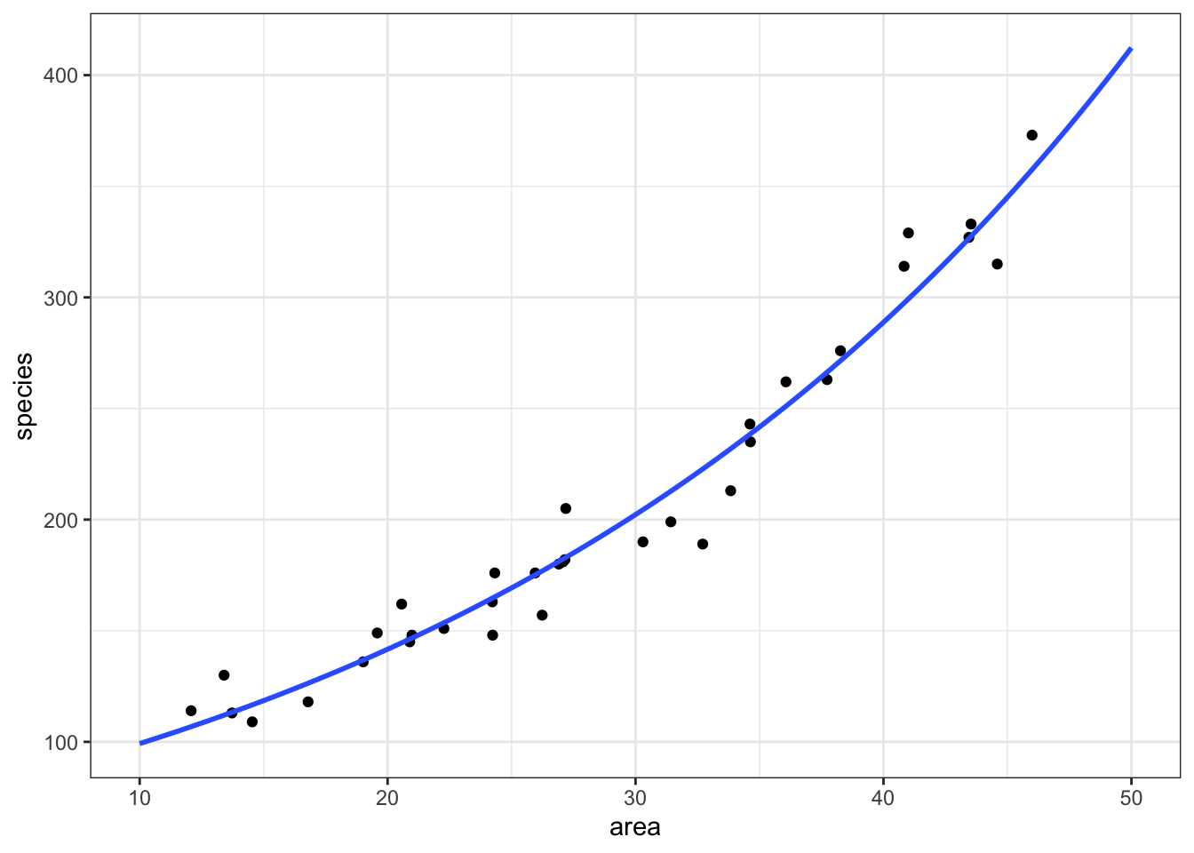

Figure 12.3: Poisson regression on species ~ area

Python

First, we produce a set of predictions, which we can then plot.

model = pd.DataFrame({'area': list(range(10, 50))})

model["pred"] = glm_isl.predict(model)

model.head()

   area        pred
0    10   99.212463
1    11  102.809432
2    12  106.536811
3    13  110.399326
4    14  114.401877

p = (ggplot(islands, aes(x = "area", y = "species")) +
   geom_point() +
   geom_line(model, aes(x = "area", y = "pred"),
                        colour = "blue", size = 1))

p.show()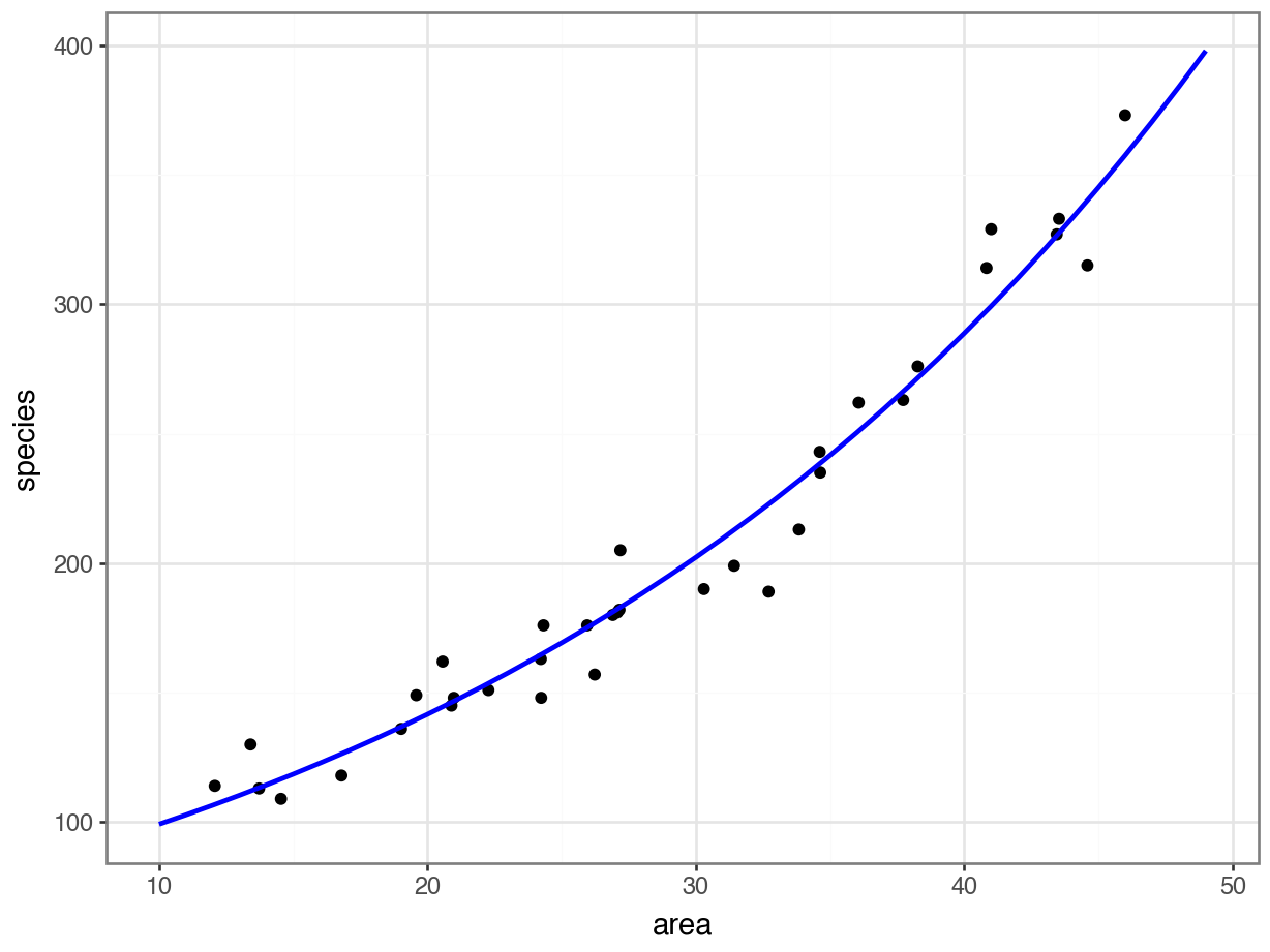

Figure 12.4: Poisson regression on species ~ area

12.6 Assumptions & model fit

As a reminder from last chapter, we want to consider the following things to assess whether we’ve fit the right model:

• The distribution of the response variable
• The link function
• Independence
• Influential points

(We don’t need to worry about collinearity here - there’s only one predictor!)

We’re also going to talk about dispersion, which really comes into play when talking about count data - we’ll get to that after we’ve run through the stuff that’s familiar.

R

With the generic check_model function, we can visually assess a few things quite quickly.

check_model(glm_isl)

Cannot simulate residuals for models of class `glm`. Please try
  `check_model(..., residual_type = "normal")` instead.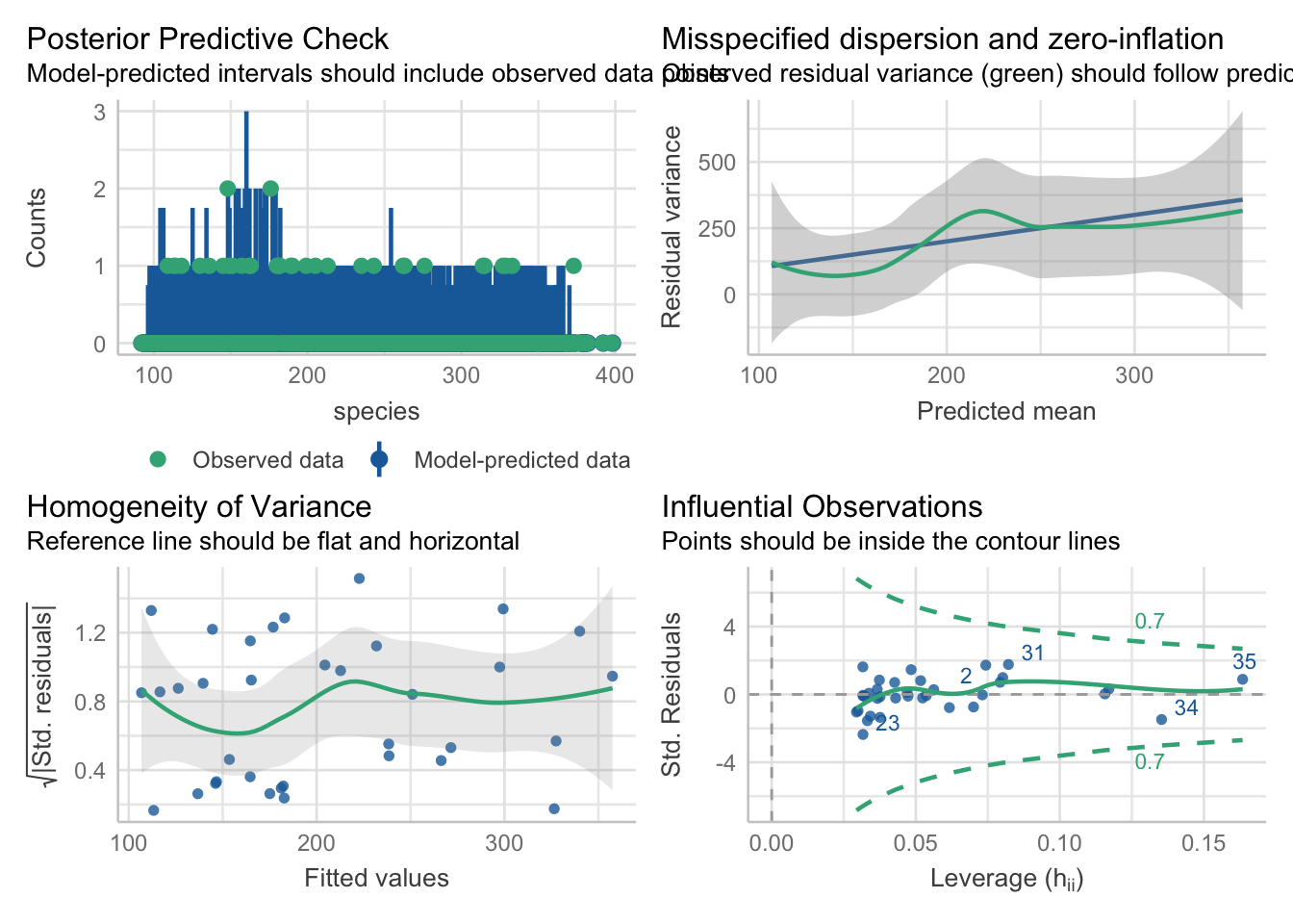

Figure 12.5: Diagnostic plots for glm_isl

The posterior predictive check looks alright. The blue simulations seem to be following a pretty similar distribution to the actual data in green.

The leverage/Cook’s distance plot also isn’t identifying any data points that we need to be concerned about. We can follow up on that:

check_outliers(glm_isl, threshold = list('cook'=0.5))

OK: No outliers detected.
- Based on the following method and threshold: cook (0.5).
- For variable: (Whole model)

Python

We can check for influential points:

influence = glm_isl.get_influence()

cooks = influence.cooks_distance[0]
influential_points = np.where(cooks > 0.5)[0]

print("Influential points:", influential_points)

Influential points: []

Influential points: There’s no evidence of any points with high Cook’s distances, so life is rosy on that front.

Independence: From the description of the dataset, it sounds plausible that each island is independent. Of course, if we later found out that some of the islands were clustered together into a bunch of archipelagos, that would definitely be cause for concern.

Distribution & link function: Again, from the description of the species variable, we can be confident that this really is a count variable. Whether or not Poisson regression with the log link function is correct, however, will depend on what happens when we look at the dispersion parameter.

12.7 Dispersion

12.7.1 What is dispersion?

Dispersion, in statistics, is a general term to describe the variability, scatter, or spread of a distribution. Variance is actually a type of dispersion.

In a normal distribution, the mean (average/central tendency) and the variance (dispersion) are independent of each other; we need both numbers, or parameters, to understand the shape of the distribution.

Other distributions, however, require different parameters to describe them in full. For a Poisson distribution - which we’ll learn more about when we talk about count data - we need just one parameter (\(\lambda\)) to describe the distribution, because the mean and variance are assumed to be the same.

In the context of a model, you can think about the dispersion as the degree to which the data are spread out around the model curve. A dispersion parameter of 1 means the data are spread out exactly as we expect; <1 is called underdispersion; and >1 is called overdispersion.

12.7.2 A “hidden assumption”

When performing Poisson regression, we make an extra assumption: that the dispersion parameter to 1. This means we don’t have to waste time and statistical power in estimating the dispersion.

However, if our data are underdispersed or overdispersed, then we might be violating this assumption we’ve made.

Underdispersion is quite rare. It’s far more likely that you’ll encounter overdispersion.

In these situations, you may wish to fit a different GLM to the data. Negative binomial regression, for instance, is a common alternative for count data.

12.7.3 Assessing dispersion

The easiest way to check dispersion in a model is to calculate the ratio of the residual deviance to the residual degrees of freedom.

If we take a look at the model output, we can see the two quantities we care about - residual deviance and residual degrees of freedom:

R

summary(glm_isl)

Call:
glm(formula = species ~ area, family = "poisson", data = islands)

Coefficients:
            Estimate Std. Error z value Pr(>|z|)    
(Intercept) 4.241129   0.041322  102.64   <2e-16 ***
area        0.035613   0.001247   28.55   <2e-16 ***
---
Signif. codes:  0 '***' 0.001 '**' 0.01 '*' 0.05 '.' 0.1 ' ' 1

(Dispersion parameter for poisson family taken to be 1)

    Null deviance: 856.899  on 34  degrees of freedom
Residual deviance:  30.437  on 33  degrees of freedom
AIC: 282.66

Number of Fisher Scoring iterations: 3

Python

print(glm_isl.summary())

                 Generalized Linear Model Regression Results                  
==============================================================================
Dep. Variable:                species   No. Observations:                   35
Model:                            GLM   Df Residuals:                       33
Model Family:                 Poisson   Df Model:                            1
Link Function:                    Log   Scale:                          1.0000
Method:                          IRLS   Log-Likelihood:                -139.33
Date:                Fri, 25 Jul 2025   Deviance:                       30.437
Time:                        08:28:47   Pearson chi2:                     30.3
No. Iterations:                     4   Pseudo R-squ. (CS):              1.000
Covariance Type:            nonrobust                                         
==============================================================================
                 coef    std err          z      P>|z|      [0.025      0.975]
------------------------------------------------------------------------------
Intercept      4.2411      0.041    102.636      0.000       4.160       4.322
area           0.0356      0.001     28.551      0.000       0.033       0.038
==============================================================================

The residual deviance is 30.44, on 33 residual degrees of freedom. All we need to do is divide one by the other to get our dispersion parameter.

R

glm_isl$deviance/glm_isl$df.residual

[1] 0.922334

Python

print(glm_isl.deviance/glm_isl.df_resid)

0.9223340414458482

The dispersion parameter here is 0.9223. That’s pretty good - not far off 1 at all.

But how can we check whether it is significantly different from 1?

R

Once again, the performance package comes in very helpful here.

The check_overdispersion function will give us both the dispersion parameter and a p-value (which is based on a chi-square test - like the goodness-of-fit ones you were running last chapter).

check_overdispersion(glm_isl)

# Overdispersion test

       dispersion ratio =  0.919
  Pearson's Chi-Squared = 30.339
                p-value =    0.6

No overdispersion detected.

Here, it confirms our suspicions; the dispersion parameter is both descriptively close to 1, and also not significantly different from 1.

You’ll notice that this function does give a slightly different value for the dispersion parameter, compared to when we calculated it manually above.

This is because it actually uses the sum of squared Pearson residuals instead of the residual deviance (a distinction which really isn’t worth worrying about). Broadly, the conclusion should be the same, so the difference doesn’t matter very much.

Python

Well, you’ve actually already got the knowledge you need to do this, from the previous chapter on significance testing.

Specifically, the chi-squared goodness-of-fit test can be used to check whether the dispersion is within sensible limits.

pvalue = chi2.sf(glm_isl.deviance, glm_isl.df_resid)

print(pvalue)

0.5953470127463268

If our chi-squared goodness-of-fit test returns a large (insignificant) p-value, as it does here, that tells us that we don’t need to worry about the dispersion.

If our chi-squared goodness-of-fit test returned a small, significant p-value, this would tell us our model doesn’t fit the data well. And, since dispersion is all about the spread of points around the model, it makes sense that these two things are so closely related!

Great - we can proceed with the Poisson regression, since we don’t seem to have overdispersed or underdispersed data.

Next chapter we’ll look at what we would have done next, if we had run into problems with dispersion.

12.8 Assessing significance

By testing the dispersion with a chi-square test, we have already essentially checked the goodness-of-fit of this model - it’s good.

This leaves us with two things to check:

1. Is the overall model better than the null model?
2. Are any of the individual predictors significant?

12.8.1 Comparing against the null

We need to fit the null model, and then we can extract the null deviance and degrees of freedom to compare against our model.

R

glm_isl_null <- glm(species ~ 1,
                    data = islands, family = "poisson")

anova(glm_isl, glm_isl_null)

Analysis of Deviance Table

Model 1: species ~ area
Model 2: species ~ 1
  Resid. Df Resid. Dev Df Deviance  Pr(>Chi)    
1        33      30.44                          
2        34     856.90 -1  -826.46 < 2.2e-16 ***
---
Signif. codes:  0 '***' 0.001 '**' 0.01 '*' 0.05 '.' 0.1 ' ' 1

Since there’s only one predictor, we actually could achieve the same effect here by just computing an analysis of deviance table:

anova(glm_isl, test = "Chisq")

Analysis of Deviance Table

Model: poisson, link: log

Response: species

Terms added sequentially (first to last)

     Df Deviance Resid. Df Resid. Dev  Pr(>Chi)    
NULL                    34     856.90              
area  1   826.46        33      30.44 < 2.2e-16 ***
---
Signif. codes:  0 '***' 0.001 '**' 0.01 '*' 0.05 '.' 0.1 ' ' 1

Python

First, we fit a null model:

model = smf.glm(formula = "species ~ 1",
                family = sm.families.Poisson(),
                data = islands)
                
glm_isl_null = model.fit()

glm_isl_null.df_resid

np.int64(34)

And now we can compare the two:

# Calculate the likelihood ratio (i.e. the chi-square value)
lrstat = -2*(glm_isl_null.llf - glm_isl.llf)

# Calculate the associated p-value
pvalue = chi2.sf(lrstat, glm_isl_null.df_resid - glm_isl.df_resid)

print(lrstat, pvalue)

826.4623291533155 9.523357725017566e-182

This gives a reported p-value extremely close to zero, which is rather small.

Therefore, this model is significant over the null, and species does appear to be predicted by area.

12.9 Exercises

12.9.1 Seat belts

Exercise 1 - Seat belts

Level:

For this exercise we’ll be using the data from data/seatbelts.csv.

The data tracks the number of drivers killed in road traffic accidents, before and after the seat belt law was introduced. The information on whether the law was in place is encoded in the law column as 0 (law not in place) or 1 (law in place).

The year variable is our predictor of interest.

In this exercise, you should:

1. Visualise the data
2. Create a poisson regression model and extract its equation
3. Plot the regression model on top of the data
4. Assess if the model is a decent predictor for the number of fatalities (& check assumptions)

R

seatbelts <- read_csv("data/seatbelts.csv")

head(seatbelts)

# A tibble: 6 × 10
  casualties drivers front  rear   kms petrol_price van_killed   law  year month
       <dbl>   <dbl> <dbl> <dbl> <dbl>        <dbl>      <dbl> <dbl> <dbl> <chr>
1        107    1687   867   269  9059        0.103         12     0  1969 Jan  
2         97    1508   825   265  7685        0.102          6     0  1969 Feb  
3        102    1507   806   319  9963        0.102         12     0  1969 Mar  
4         87    1385   814   407 10955        0.101          8     0  1969 Apr  
5        119    1632   991   454 11823        0.101         10     0  1969 May  
6        106    1511   945   427 12391        0.101         13     0  1969 Jun  

Python

seatbelts = pd.read_csv("data/seatbelts.csv")

seatbelts.head()

   casualties  drivers  front  rear  ...  van_killed  law  year  month
0         107     1687    867   269  ...          12    0  1969    Jan
1          97     1508    825   265  ...           6    0  1969    Feb
2         102     1507    806   319  ...          12    0  1969    Mar
3          87     1385    814   407  ...           8    0  1969    Apr
4         119     1632    991   454  ...          10    0  1969    May

[5 rows x 10 columns]

Answer

Visualise the data

First we have a look at the data comparing no law versus law:

R

We have to convert the law column to a factor, otherwise R will see it as numerical.

seatbelts |> 
  ggplot(aes(as_factor(law), casualties)) +
   geom_boxplot() +
   geom_jitter(width = 0.2)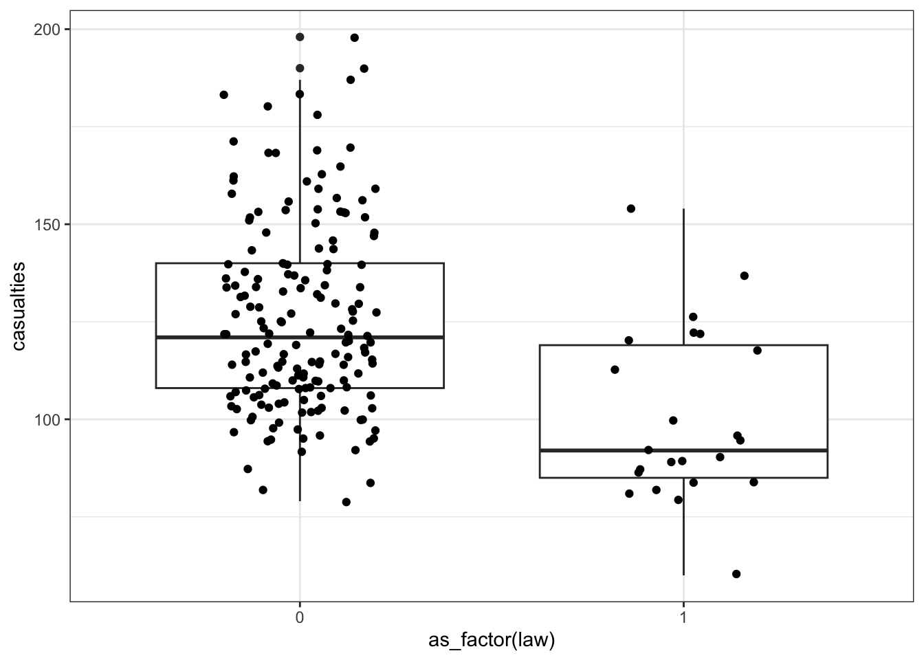

Figure 12.6: Boxplot of driver casualties before and after seatbelt introduction

The data are recorded by month and year, so we can also display the number of drivers killed by year:

seatbelts |> 
  ggplot(aes(year, casualties)) +
  geom_point()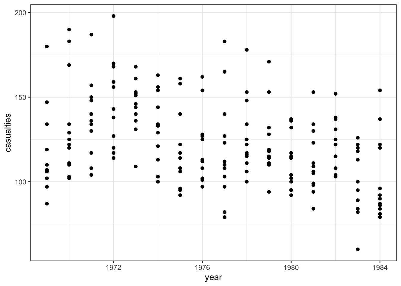

Figure 12.7: Scatterplot of driver casualties across years

Python

We have to convert the law column to a factor, otherwise R will see it as numerical.

p = (ggplot(seatbelts, aes(x = seatbelts.law.astype(object),
                       y = "casualties")) +
   geom_boxplot() +
   geom_jitter(width = 0.2))

p.show()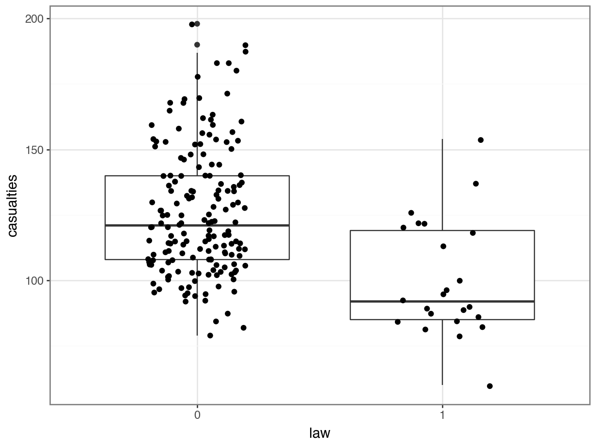

Figure 12.8: Boxplot of driver casualties before and after seatbelt introduction

The data are recorded by month and year, so we can also display the number of casualties by year:

p = (ggplot(seatbelts,
         aes(x = "year",
             y = "casualties")) +
     geom_point())

p.show()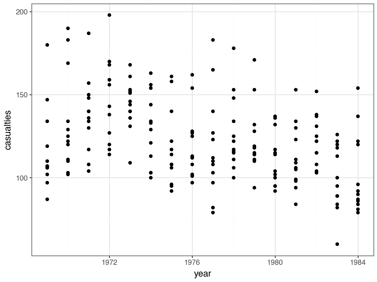

Figure 12.9: Scatterplot of driver casualties across years

The data look a bit weird. There’s a bit of a wavy pattern across years. And although it looks like fatalities are lower after the law was implemented, there are many more observations when the law was not in place, which is going to make the data harder to interpret.

Constructing a model

R

glm_stb <- glm(casualties ~ year,
               data = seatbelts, family = "poisson")

Python

model = smf.glm(formula = "casualties ~ year",
                family = sm.families.Poisson(),
                data = seatbelts)

glm_stb = model.fit()

Model equation

R

coefficients(glm_stb)

(Intercept)        year 
  37.168958   -0.016373 

Python

print(glm_stb.params)

Intercept    37.168958
year         -0.016373
dtype: float64

The coefficients of the Poisson model equation should be placed in the following formula, in order to estimate the expected number of species as a function of island size:

\[ E(casualties) = \exp(37.17 - -0.016 \times year) \]

Visualise model

We can just adapt the code used in the worked example earlier in the chapter:

R

ggplot(seatbelts, aes(year, casualties)) +
  geom_point() +
  geom_smooth(method = "glm", se = FALSE, fullrange = TRUE, 
              method.args = list(family = poisson)) +
  xlim(1970, 1985)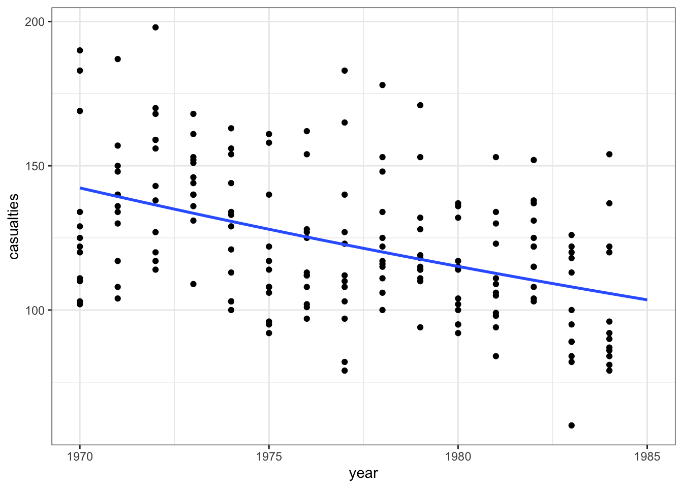

Figure 12.10: Poisson regression of driver casualties across years

Python

model = pd.DataFrame({'year': list(range(1968, 1985))})

model["pred"] = glm_stb.predict(model)

model.head()

   year        pred
0  1968  140.737690
1  1969  138.452153
2  1970  136.203733
3  1971  133.991827
4  1972  131.815842

p = (ggplot(seatbelts, aes(x = "year",
                       y = "casualties")) +
   geom_point() +
   geom_line(model, aes(x = "year", y = "pred"),
                        colour = "blue", size = 1))

p.show()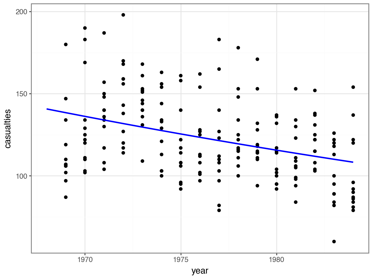

Figure 12.11: Poisson regression of driver casualties across years

Assessing model quality & significance

Are the assumptions met?

Response distribution & link function	Yes, based on the info given
Independence	Yes, based on the info given
Influential points	Check with Cook’s distance
Dispersion	Check dispersion parameter

R

We can assess outliers visually or by printing a list of high leverage points:

check_outliers(glm_stb, threshold = list('cook'=0.5))

OK: No outliers detected.
- Based on the following method and threshold: cook (0.5).
- For variable: (Whole model)

check_model(glm_stb, check = 'outliers')

Cannot simulate residuals for models of class `glm`. Please try
  `check_model(..., residual_type = "normal")` instead.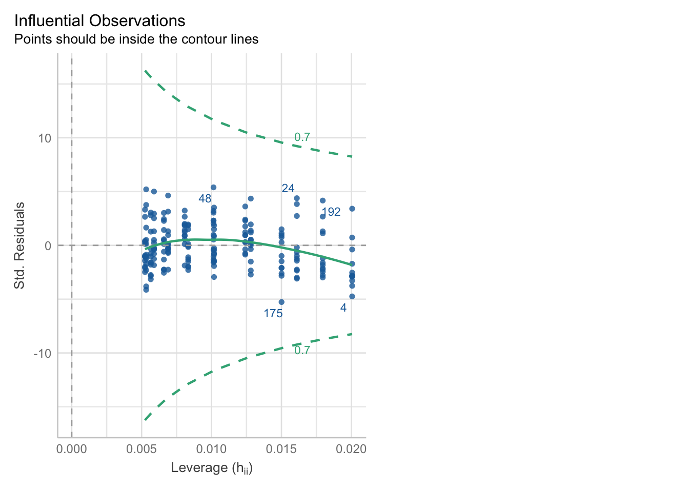

It seems we’re okay on the outlier front.

For dispersion, again we have some options of how to test it:

check_overdispersion(glm_stb)

# Overdispersion test

       dispersion ratio =   4.535
  Pearson's Chi-Squared = 861.667
                p-value = < 0.001

Overdispersion detected.

check_model(glm_stb, check = 'overdispersion')

Cannot simulate residuals for models of class `glm`. Please try
  `check_model(..., residual_type = "normal")` instead.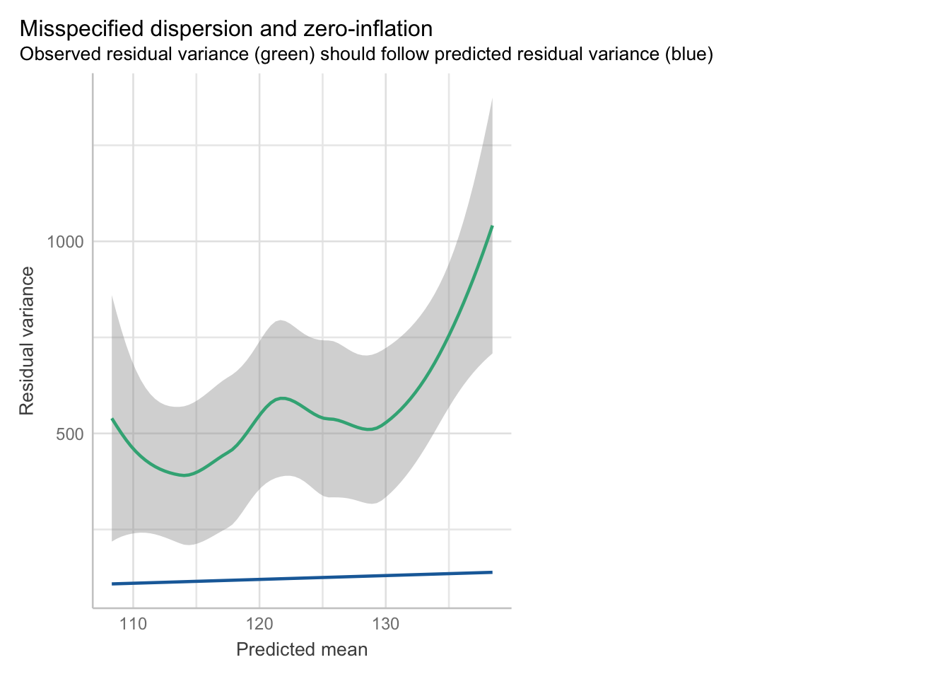

Dispersion is definitely a problem here.

For completeness, we can also peek at the posterior predictive check:

check_model(glm_stb, check = 'pp_check')

Cannot simulate residuals for models of class `glm`. Please try
  `check_model(..., residual_type = "normal")` instead.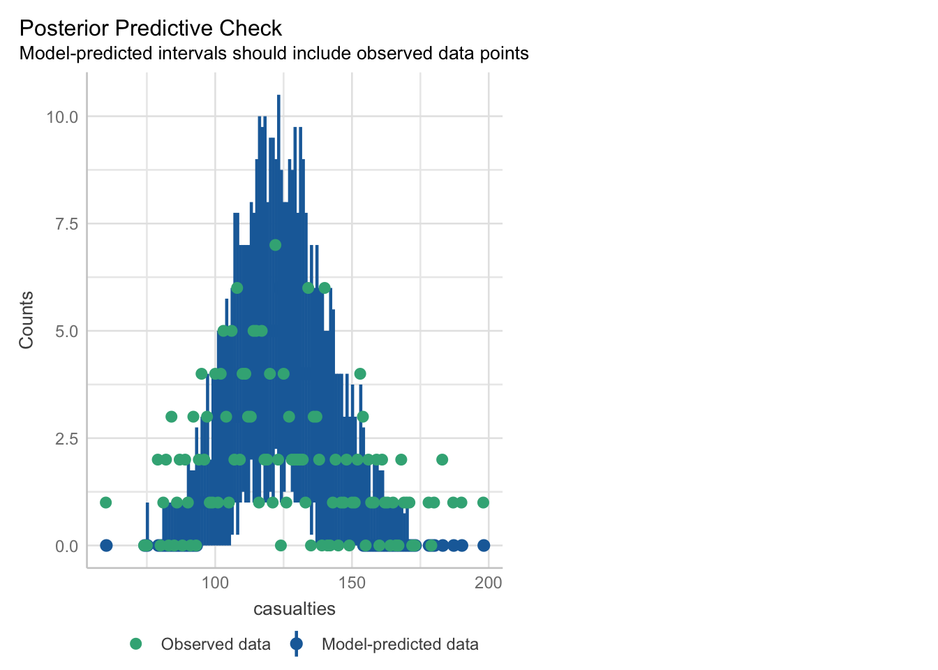

It doesn’t seem to be doing the best job. Around 0 and in the 180+ range of the x-axis, it’s under-predicting the counts; and it might be over-predicting a bit in the middle (120-140 ish).

Python

We can assess outliers by printing a list of high leverage points:

influence = glm_isl.get_influence()

cooks = influence.cooks_distance[0]
influential_points = np.where(cooks > 0.5)[0]

print("Influential points:", influential_points)

Influential points: []

It seems we’re okay on the outlier front.

For dispersion, let’s calculate the parameter and p-value:

pvalue = chi2.sf(glm_stb.deviance, glm_stb.df_resid)

print(glm_stb.deviance/glm_stb.df_resid, pvalue)

4.475851158209689 3.1298697149299994e-84

Dispersion is definitely a problem here.

Response distribution & link function	Yes, based on the info given
Independence	Yes, based on the info given
Influential points	Yes, no data points identified
Dispersion	Clear overdispersion

Given that we have a problem with overdispersion, we probably wouldn’t proceed with significance testing here under normal circumstances. Instead, we’d want to fit a different GLM that can handle this overdispersion.

For completeness, however, since these are course materials rather than normal circumstances - let’s check: is the model significant over the null?

R

glm_null <- glm(casualties ~ 1, 
                family = "poisson", 
                data = seatbelts)

anova(glm_stb, glm_null)

Analysis of Deviance Table

Model 1: casualties ~ year
Model 2: casualties ~ 1
  Resid. Df Resid. Dev Df Deviance  Pr(>Chi)    
1       190     850.41                          
2       191     984.50 -1  -134.08 < 2.2e-16 ***
---
Signif. codes:  0 '***' 0.001 '**' 0.01 '*' 0.05 '.' 0.1 ' ' 1

Python

model = smf.glm(formula = "casualties ~ 1",
                family = sm.families.Poisson(),
                data = seatbelts)

glm_stb_null = model.fit()

lrstat = -2*(glm_stb_null.llf - glm_stb.llf)
pvalue = chi2.sf(lrstat, glm_stb_null.df_resid - glm_stb.df_resid)

print(lrstat, pvalue)

134.0834016068129 5.23879166948147e-31

What does the significant p-value here tell us?

Well, given the difference in degrees of freedom (1), the change in residual deviance between our model and the null model is unexpectedly large. So the model is doing something over and above what the null is doing.

Conclusions

Does this significant comparison against the null allow us to draw any conclusions about whether the seatbelt law affects the number of casualties?

No. Don’t let it tempt you.

The model we’ve constructed here is not a good fit and doesn’t meet all of the assumptions. We need to fit a different type of model that can cope with the overdispersion, which we’ll look into next chapter.

12.10 Summary

Key points

• Count data are bounded between 0 and \(\infty\), with integer increases
• This type of data can be modelled with a Poisson regression, using a log link function
• Poisson regression makes all of the same assumptions as logistic regression, plus an assumption about dispersion