11 Checking assumptions

Learning outcomes

Know what statistical assumptions apply to logistic regression (and GLMs)
Be able to evaluate whether a logistic regression meets the assumptions

11.1 Context

We can now assess the quality of a generalised linear model. Although we can relax certain assumptions compared to standard linear models (linearity, equality of variance of residuals, and normality of residuals), we cannot relax all of them - some key assumptions still exist. We discuss these below.

11.2 Section setup

Click to expand

We’ll use the following libraries and data:

R
Python

# Load required R libraries
library(tidyverse)
library(ggResidpanel)
library(performance)

# Read in the required data
diabetes <- read_csv("data/diabetes.csv")
levers <- read_csv("data/levers.csv")
seeds <- read_csv("data/seeds.csv")

# Load required Python libraries
import pandas as pd
import numpy as np
import matplotlib.pyplot as plt
import statsmodels.api as sm
import statsmodels.formula.api as smf
from statsmodels.stats.outliers_influence import variance_inflation_factor
from patsy import dmatrix
from scipy.stats import *
from plotnine import *

# Read in the required data
diabetes = pd.read_csv("data/diabetes.csv")
levers = pd.read_csv("data/levers.csv")
seeds = pd.read_csv("data/seeds.csv")

11.3 Assumption checking

Below we go through the various assumptions we need to consider.

11.3.1 Assumption 1: Distribution of response variable

Although we don’t expect our response variable \(y\) to be continuous and normally distributed (as we did in linear modelling), we do still expect its distribution to come from the “exponential family” of distributions.

The exponential family

The exponential family contains the following distributions, among others:

normal
exponential
Poisson
Bernoulli
binomial (for fixed number of trials)
chi-squared

You can use a histogram to visualise the distribution of your response variable, but it is typically most useful just to think about the nature of your response variable. For instance, binary variables will follow a Bernoulli distribution, proportional variables follow a binomial distribution, and most count variables will follow a Poisson distribution.

If you have a very unusual variable that doesn’t follow one of these exponential family distributions, however, then a GLM will not be an appropriate choice. In other words, a GLM is not necessarily a magic fix!

11.3.2 Assumption 2: Correct link function

A closely-related assumption to assumption 1 above, is that we have chosen the correct link function for our model.

If we have done so, then there should be a linear relationship between our transformed model and our response variable; in other words, if we have chosen the right link function, then we have correctly “linearised” our model.

11.3.3 Assumption 3: Independence

We expect that the each observation or data point in our sample is independent of all the others. Specifically, we expect that our set of \(y\) response variables are independent of one another.

For this to be true, we have to make sure:

that we aren’t treating technical replicates as true/biological replicates;
that we don’t have observations/data points in our sample that are artificially similar to each other (compared to other data points);
that we don’t have any nuisance/confounding variables that create “clusters” or hierarchy in our dataset;
that we haven’t got repeated measures, i.e., multiple measurements/rows per individual in our sample

There is no diagnostic plot for assessing this assumption. To determine whether your data are independent, you need to understand your experimental design.

You might find this page useful if you’re looking for more information on what counts as truly independent data.

11.4 Other features to check

There are a handful of other features or qualities that can affect the quality of model fit, and therefore the quality of the inferences we draw from it.

These are not necessarily “formal” assumptions, but it’s good practice to check for them.

Lack of influential observations

A data point is overly influential, i.e., has high leverage, if removing that point from the dataset would cause large changes in the model coefficients. Data points with high leverage are typically those that don’t follow the same general “trend” as the rest of the data.

Lack of collinearity

Collinearity is when predictor variables are overly/strongly correlated with each other. This can make it very difficult to estimate the right beta coefficients and individual p-values for those predictors.

Dispersion

This is mentioned here for completeness, and as a bit of sizzle for next chapter when we talk about Poisson regression.

We won’t be worrying about dispersion in logistic regression specifically.

If you want more detail, you can skip ahead now to Section 12.7.

11.5 Assessing assumptions & quality

In linear modelling, we rely heavily on visuals to determine whether various assumptions were met.

When checking assumptions and assessing quality of fit for GLMs, we don’t use the panel of diagnostic plots that we used for linear models any more. However, there are some visualisations that can help us, plus several metrics we can calculate from our data or model.

	Is it a formal assumption?	How can I assess it?
Response variable comes from a distribution in the exponential family & The model uses the right link function	Yes	Knowledge of the experimental design Some plots, e.g., posterior predictive check/uniform Q-Q, may help
Independent observations	Yes	Knowledge of experimental design There are no formal tests or plots that assess independence reliably
Influential observations	No	Cook’s distance/leverage plot
Lack of collinearity	No	Variance inflation factor
Dispersion	Sort of	Calculating the dispersion parameter Can also be visualised

R
Python

diabetes <- read_csv("data/diabetes.csv")

glm_dia <- glm(test_result ~ glucose * diastolic,
                  family = "binomial",
                  data = diabetes)

Let’s fit some useful diagnostic plots, using the diabetes and aphids example datasets.

We’re going to rely heavily on the performance package in R for assessing the assumptions and fit of our model.

The check_model function will be our primary workhorse. This function automatically detects the type of model you give it, and produces the appropriate panel of plots all by itself. (So, so cool. And yes, it works for linear models too!)

check_model(glm_dia)

Cannot simulate residuals for models of class `glm`. Please try
  `check_model(..., residual_type = "normal")` instead.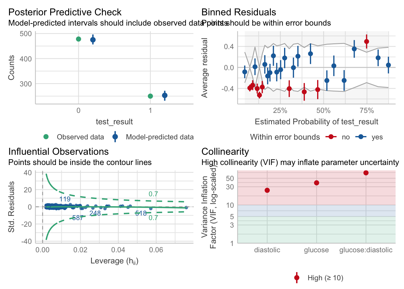

Figure 11.1: Diagnostic plots for the `glm_dia` model

Creating diagnostic plots in Python is not straightforward, since there are no decent packages out there. However, that does not mean we can’t check assumptions! In the next few sections we’ll visit every assumption individually using code.

If you’re interested in the visual aspect, just look at the R code.

We’ll start with creating the model.

diabetes_py = pd.read_csv("data/diabetes.csv")

model = smf.glm(formula = "test_result ~ glucose * diastolic",
                family = sm.families.Binomial(),
                data = diabetes_py)

glm_dia_py = model.fit()

We can check for outliers via a leverage plot (in performance), which you may remember from linear modelling.

Ideally, data points would fall inside the green contour lines. Data points that don’t will be highlighted in red.

check_model(glm_dia, check = 'outliers')

Cannot simulate residuals for models of class `glm`. Please try
  `check_model(..., residual_type = "normal")` instead.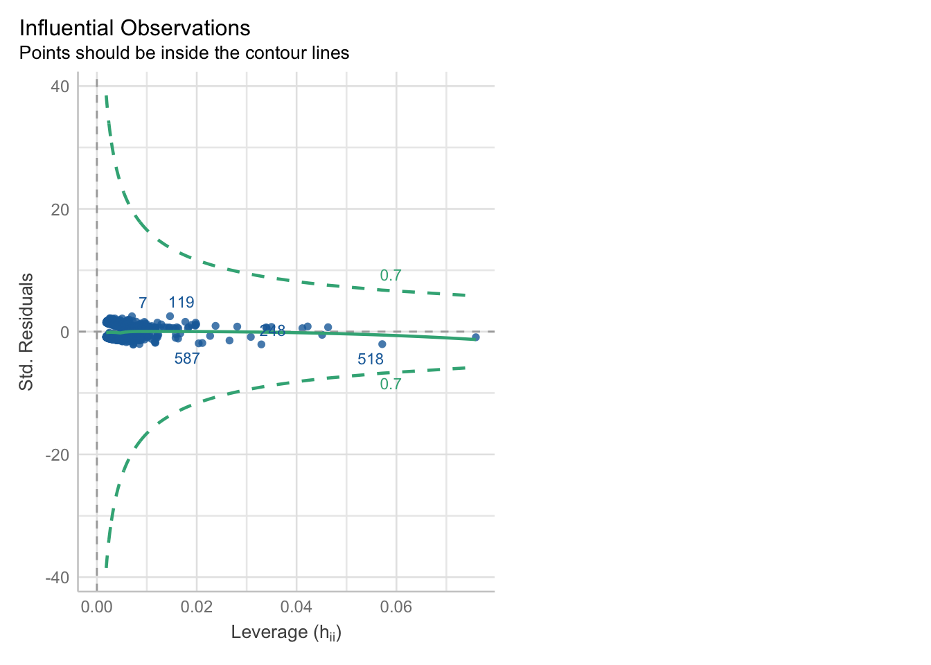

Figure 11.2: Influential points check for `glm_dia` model

Alternatively, we can use the check_outliers function:

check_outliers(glm_dia, threshold = list('cook' = 0.5))

OK: No outliers detected.
- Based on the following method and threshold: cook (0.5).
- For variable: (Whole model)

That said, this is the one plot we can create quite easily: Cook’s D.

We can use the get_influence function to extract information like leverage, Cook’s distance etc. about all of our data points:

# extract the Cook's distances
glm_dia_py_resid = pd.DataFrame(glm_dia_py.
                                get_influence().
                                summary_frame()["cooks_d"])

# add row index 
glm_dia_py_resid['obs'] = glm_dia_py_resid.reset_index().index

We now have two columns:

glm_dia_py_resid.head()

    cooks_d  obs
0  0.000709    0
1  0.000069    1
2  0.000641    2
3  0.000080    3
4  0.009373    4

We can use these to create the plot:

p = (ggplot(glm_dia_py_resid,
         aes(x = "obs",
             y = "cooks_d")) +
     geom_segment(aes(x = "obs", y = "cooks_d", xend = "obs", yend = 0)) +
     geom_point())

p.show()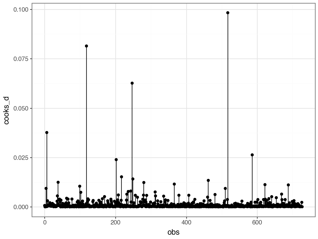

Figure 11.3: Influential points check for `glm_dia_py` model

Alternative method using matplotlib

influence = glm_dia_py.get_influence()

Then, we can visualise and interrogate that information.

We can produce a Cook’s distance plot (this uses matplotlib):

cooks = influence.cooks_distance[0]

plt.stem(np.arange(len(cooks)), cooks, markerfmt=",")
plt.axhline(0.5, color='red', linestyle='--', label='Threshold')
plt.xlabel('Observation')
plt.ylabel("Cook's Distance")
plt.title("Cook's Distance Plot")
plt.legend()
plt.show()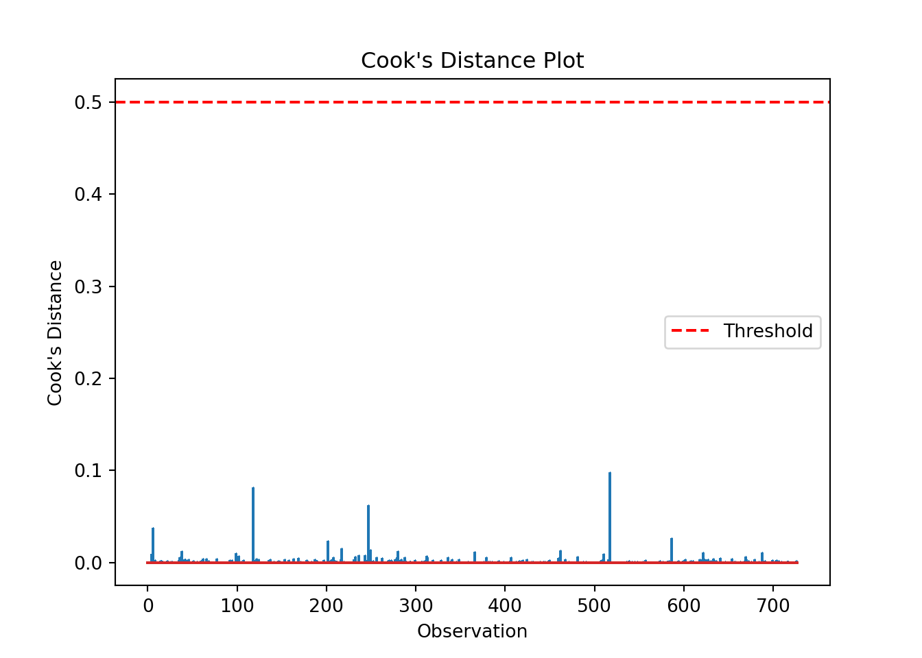

Figure 11.4: Influential points check for `glm_dia_py` model

and/or we can extract a list of data points with a Cook’s distance greater than some specified threshold:

influential_points = np.where(cooks > 0.5)[0] # Set appropriate threshold here

print("Influential points:", influential_points)

Influential points: []

The list is empty, indicating no high leverage points that we need to worry about.

We can check which points may be influential, for example by setting a threshold of > 0.5:

influential_points = glm_dia_py_resid[glm_dia_py_resid["cooks_d"] > 0.5]

print("Influential points:", influential_points)

Influential points: Empty DataFrame
Columns: [cooks_d, obs]
Index: []

The DataFrame is empty, indicating no high leverage points that we need to worry about.

Dealing with “outliers”

Remember:

Outliers and influential points aren’t necessarily the same thing; all outliers need to be followed up, to check if they are influential in a problematic way
You can’t just drop data points because they are inconvenient! This is cherry-picking, and it can impact the quality and generalisability of your conclusions

11.5.2 Lack of collinearity

The best way to assess whether we have collinearity is to look at something called the variance inflation factor (VIF).

When calculating VIF for a model, a separate VIF value will be generated for each predictor. VIF >5 is worth an eyebrow raise; VIF >10 definitely needs some follow-up; and VIF >20 suggests a really strong correlation that is definitely problematic.

R
Python

check_collinearity(glm_dia)

Model has interaction terms. VIFs might be inflated.
  Try to center the variables used for the interaction, or check
  multicollinearity among predictors of a model without interaction terms.

# Check for Multicollinearity

High Correlation

              Term   VIF     VIF 95% CI adj. VIF Tolerance Tolerance 95% CI
           glucose 37.99 [32.97, 43.80]     6.16      0.03     [0.02, 0.03]
         diastolic 24.24 [21.06, 27.92]     4.92      0.04     [0.04, 0.05]
 glucose:diastolic 69.45 [60.21, 80.14]     8.33      0.01     [0.01, 0.02]

We can also visualise the VIFs, if we prefer, with the VIF plot in check_model:

check_model(glm_dia, check = "vif")

Cannot simulate residuals for models of class `glm`. Please try
  `check_model(..., residual_type = "normal")` instead.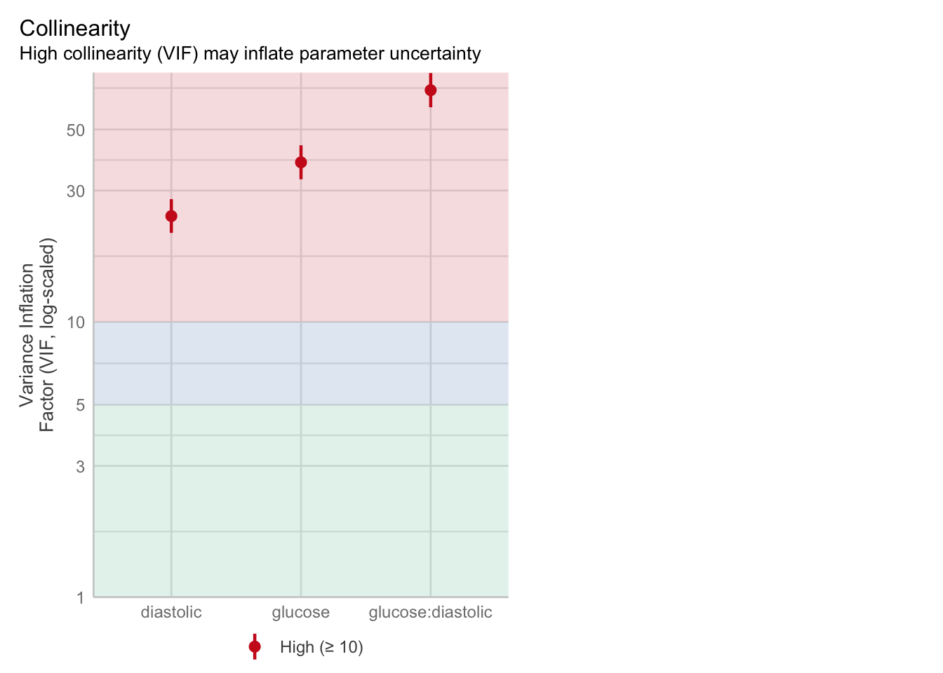

Figure 11.5: Collinearity check for `glm_dia` model

The statsmodels package contains a function for calculating VIF.

It uses the original data, rather than the model, to do this. This means you have to manually exclude the response variable, and then use the dmatrix function from patsy to create the matrix that can be used to calculate the VIF.

from statsmodels.stats.outliers_influence import variance_inflation_factor
from patsy import dmatrix

# Drop the response variable
X = diabetes_py.drop(columns='test_result')

# Create design matrix based on model formula
X = dmatrix("glucose * diastolic", data=diabetes_py, return_type='dataframe')

# Calculate VIF for each feature
vif_data = pd.DataFrame()
vif_data['feature'] = X.columns
vif_data['VIF'] = [variance_inflation_factor(X.values, i)
                   for i in range(X.shape[1])]

print(vif_data)

             feature         VIF
0          Intercept  600.539179
1            glucose   36.879125
2          diastolic   17.407953
3  glucose:diastolic   63.987700

There is definitely some collinearity going on in our model - these VIF values are way over 10.

The most likely culprit for this is the interaction term - let’s see if we can improve things by dropping it:

R
Python

glm_dia_add <- glm(test_result ~ glucose + diastolic,
                  family = "binomial",
                  data = diabetes)

check_collinearity(glm_dia_add)

# Check for Multicollinearity

Low Correlation

      Term  VIF   VIF 95% CI adj. VIF Tolerance Tolerance 95% CI
   glucose 1.02 [1.00, 1.78]     1.01      0.98     [0.56, 1.00]
 diastolic 1.02 [1.00, 1.78]     1.01      0.98     [0.56, 1.00]

check_model(glm_dia_add, check = "vif")

Cannot simulate residuals for models of class `glm`. Please try
  `check_model(..., residual_type = "normal")` instead.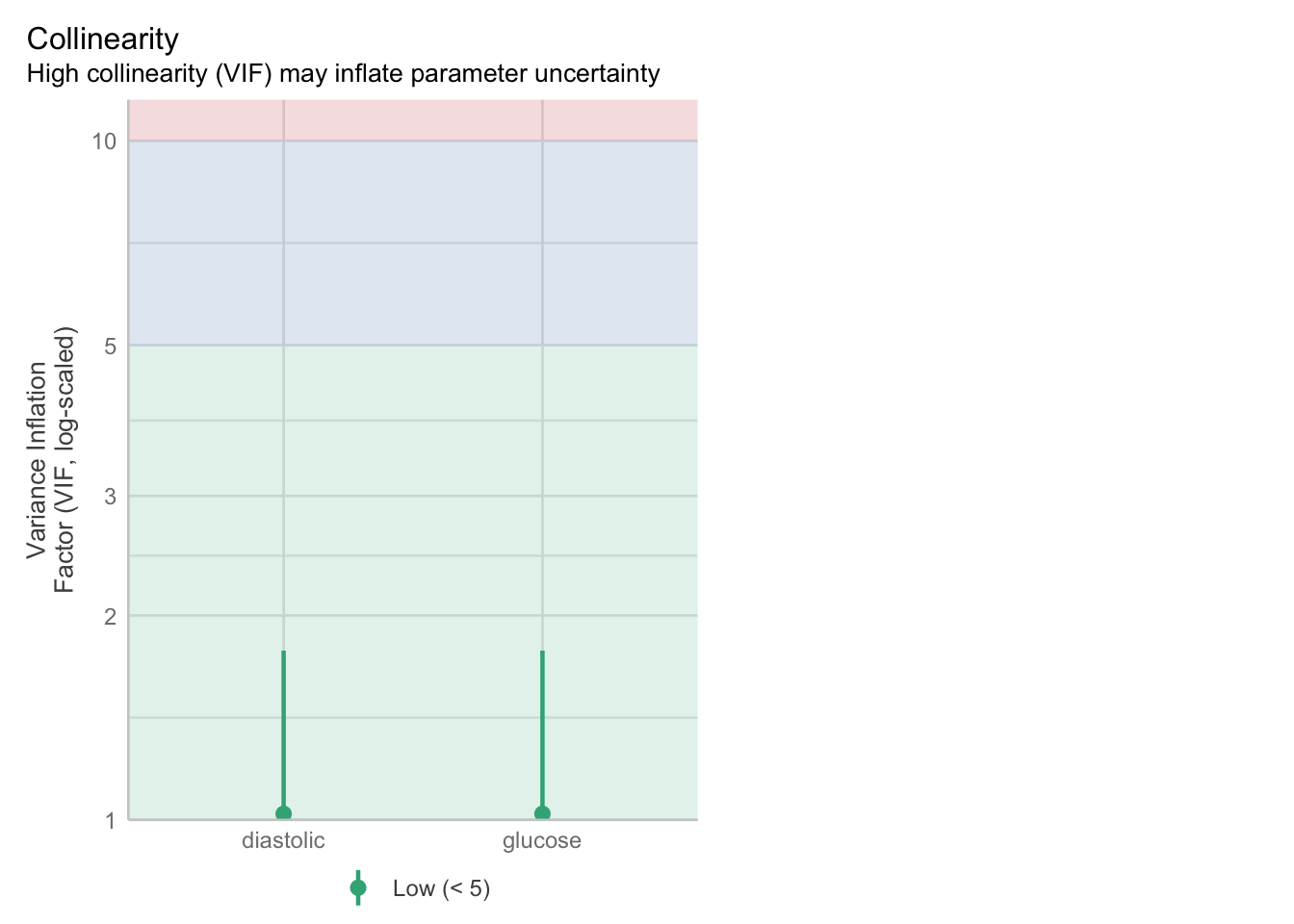

Figure 11.6: Collinearity check for `glm_dia_add` model

We will try again, this time without manually adding the interaction:

# 1. Drop the response variable
X = diabetes_py.drop(columns='test_result')

# 2. Add constant column for intercept
X = sm.add_constant(X)

# Calculate VIF for each feature
vif_data = pd.DataFrame()
vif_data['feature'] = X.columns
vif_data['VIF'] = [variance_inflation_factor(X.values, i)
                   for i in range(X.shape[1])]

print(vif_data)

     feature        VIF
0      const  42.747425
1    glucose   1.052426
2  diastolic   1.052426

Much better! This means that dropping the interaction term drastically improves the model.

Why does this matter? Well, if you want to make specific comments about the predictors, then collinearity is an issue, because dropping one of the predictors can cause large swings in the beta estimates. This is an issue if you try to have a meaningful model.

If all you care about is the overall accuracy of your model (the machine learning approach, where all we care about is maximum prediction) then collinearity becomes irrelevant, because the model and residuals don’t change due to collinearity.

11.6 Exercises

11.6.1 Revisiting rats and levers (again)

Exercise 1 - Revisiting rats and levers (again)

Level:

In Exercise 8.7.1 and Exercise 9.7.3, you worked through the levers dataset, fitting an appropriate model and then assessing its significance.

Now, using what you’ve learned in this chapter, assess whether this logistic regression is appropriate:

R
Python

levers <- read_csv("data/levers.csv")

levers <- levers |> 
  mutate(incorrect_presses = trials - correct_presses)

glm_lev <- glm(cbind(correct_presses, incorrect_presses) ~ stress_type * sex + rat_age,
               family = binomial,
               data = levers)

levers = pd.read_csv("data/levers.csv")

levers['incorrect_presses'] = levers['trials'] - levers['correct_presses']

model = smf.glm(formula = "correct_presses + incorrect_presses ~ stress_type * sex + rat_age",
                family = sm.families.Binomial(),
                data = levers)

glm_lev = model.fit()

Answer

Consider the response variable

Is a logistic regression, with a logit link function, appropriate?

For the answer to be “yes”, then our response variable needs to be either a binary or a proportional variable (binomially distributed). We’re looking for those success/fail trials.

Sometimes, it can help to visualise the design:

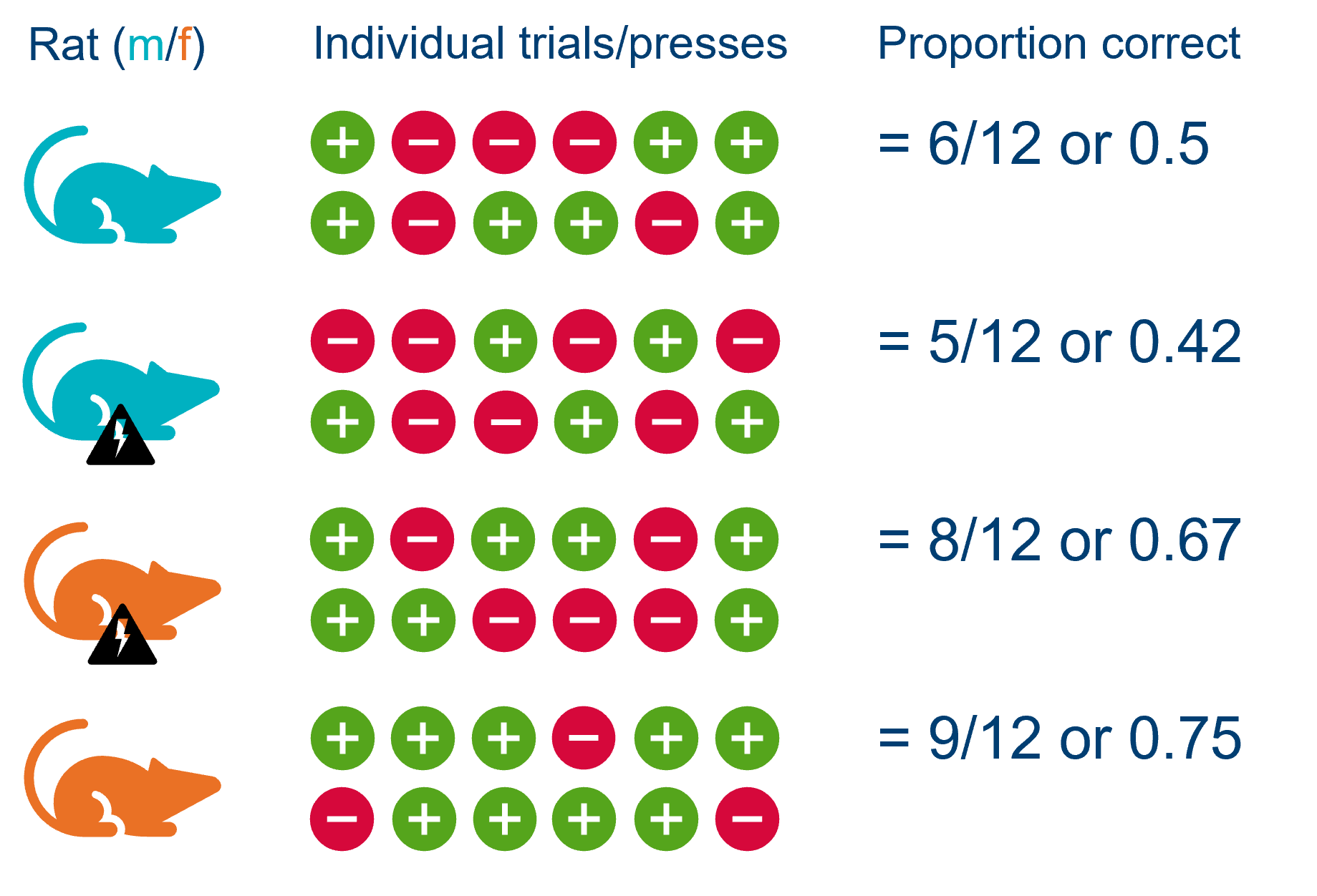
Experimental design for rat lever experiment

We can see that for each rat, the proportion score is made up of a series of trials, each of which can either be correct (+) or incorrect (-).

Consider independence

Again, we need to think about the design.

It might initially seem as if we have multiple observations per animal - since each rat pressed a whole bunch of levers - but actually if we look at each row of our dataset:

R
Python

head(levers)

# A tibble: 6 × 8
  rat_id stress_type sex    rat_age trials correct_presses prop_correct
   <dbl> <chr>       <chr>    <dbl>  <dbl>           <dbl>        <dbl>
1      1 control     female      13     20               7         0.35
2      2 control     female      15     20              11         0.55
3      3 control     female      11     20               5         0.25
4      4 control     female      15     20               5         0.25
5      5 stressed    female      13     20               8         0.4 
6      6 stressed    male        14     20               8         0.4 
# ℹ 1 more variable: incorrect_presses <dbl>

levers.head()

   rat_id stress_type     sex  ...  correct_presses  prop_correct  incorrect_presses
0       1     control  female  ...                7          0.35                 13
1       2     control  female  ...               11          0.55                  9
2       3     control  female  ...                5          0.25                 15
3       4     control  female  ...                5          0.25                 15
4       5    stressed  female  ...                8          0.40                 12

[5 rows x 8 columns]

it becomes clear that each row of the dataset represents a rat, rather than each row representing a separate trial/button press.

In other words: by collecting the proportion of correct trials, we have averaged across the rat, and so it only appears once in our dataset.

This means that each of the rows of the dataset truly are independent.

Now, this does make some assumptions about the nature of the rats’ relationships to each other. Some non-independence could be introduced if:

Some of the rats are genetically more similar to each other, e.g., if multiple rats from the same litter were included
Rats were trained together before testing
Rats were exposed to stress in one big batch (i.e., putting them all in one cage with the smell of a predator) rather than individually

Influential observations

R
Python

check_model(glm_lev, check = 'outliers')

Cannot simulate residuals for models of class `glm`. Please try
  `check_model(..., residual_type = "normal")` instead.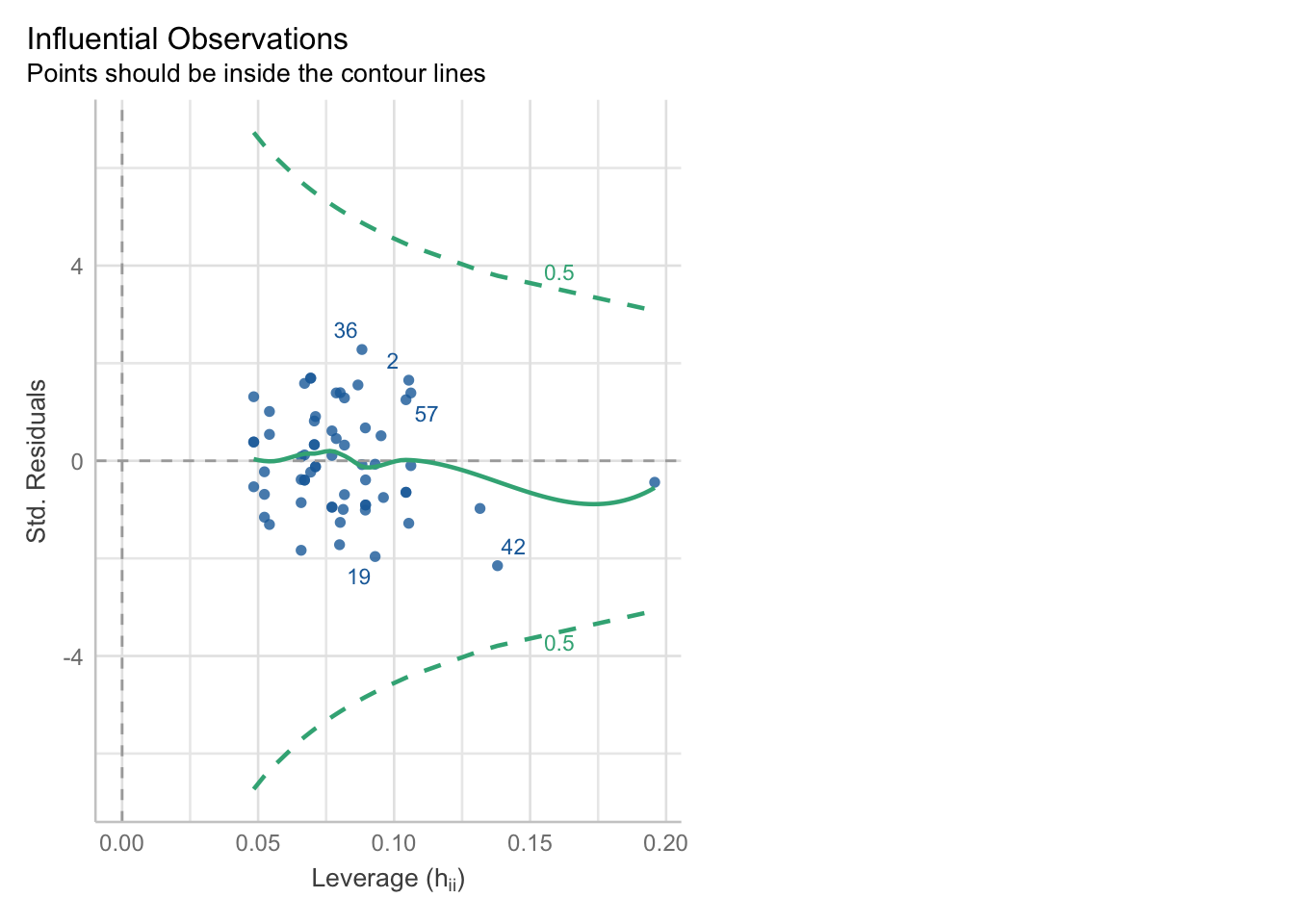

check_outliers(glm_lev)

OK: No outliers detected.
- Based on the following method and threshold: cook (0.5).
- For variable: (Whole model)

influence = glm_lev.get_influence()

cooks = influence.cooks_distance[0]

plt.stem(np.arange(len(cooks)), cooks, markerfmt=",")
plt.axhline(0.5, color='red', linestyle='--', label='Threshold')
plt.xlabel('Observation')
plt.ylabel("Cook's Distance")
plt.title("Cook's Distance Plot")
plt.legend()
plt.show()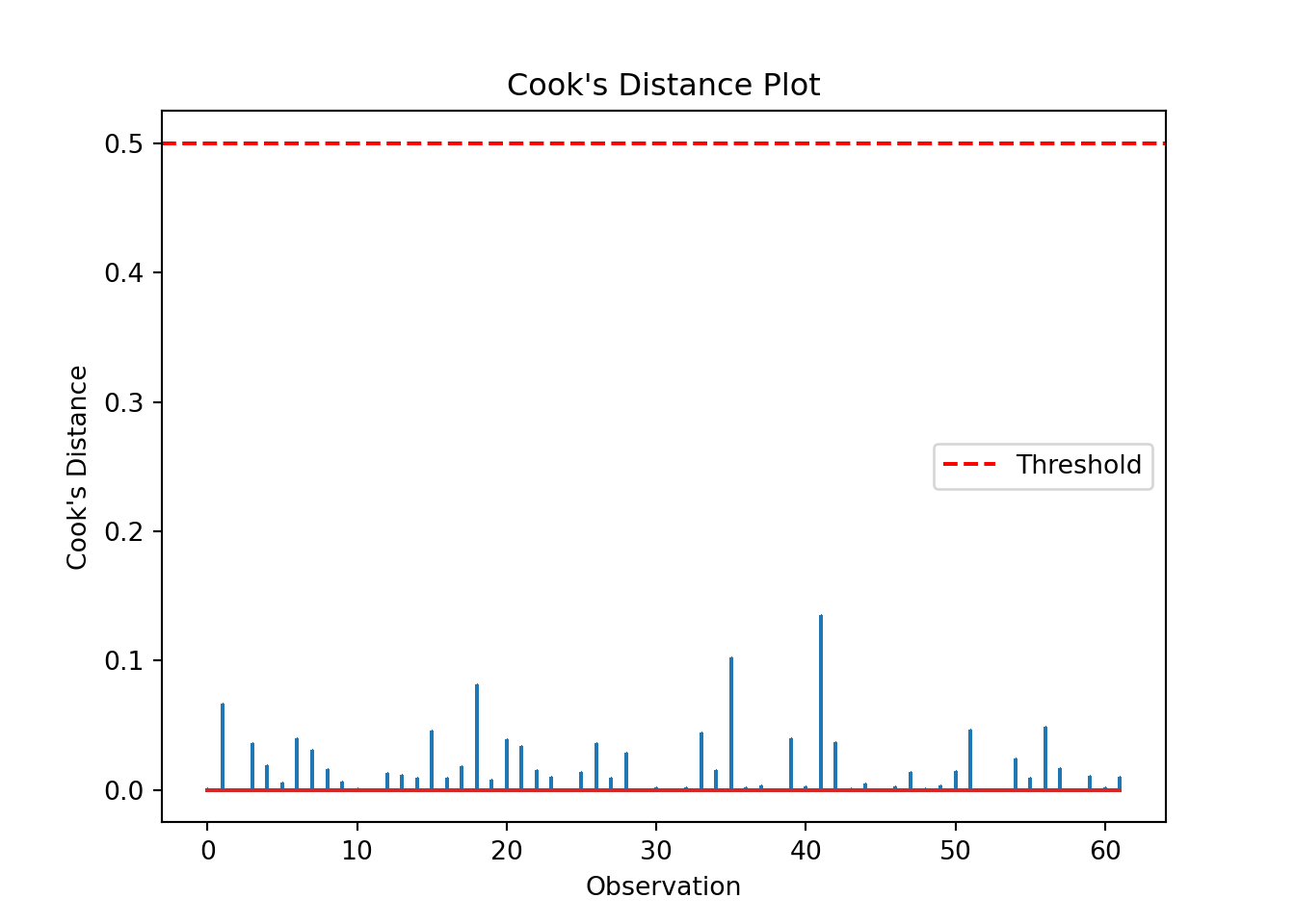

influential_points = np.where(cooks > 0.5)[0] # Set appropriate threshold here

print("Influential points:", influential_points)

Influential points: []

Looks good!

Collinearity

R
Python

check_collinearity(glm_lev)

# Check for Multicollinearity

Low Correlation

            Term  VIF     VIF 95% CI adj. VIF Tolerance Tolerance 95% CI
     stress_type 1.81 [1.40,   2.64]     1.34      0.55     [0.38, 0.72]
             sex 2.23 [1.66,   3.28]     1.49      0.45     [0.30, 0.60]
         rat_age 1.02 [1.00, 287.92]     1.01      0.98     [0.00, 1.00]
 stress_type:sex 2.70 [1.97,   4.01]     1.64      0.37     [0.25, 0.51]

check_model(glm_lev, check = "vif")

Cannot simulate residuals for models of class `glm`. Please try
  `check_model(..., residual_type = "normal")` instead.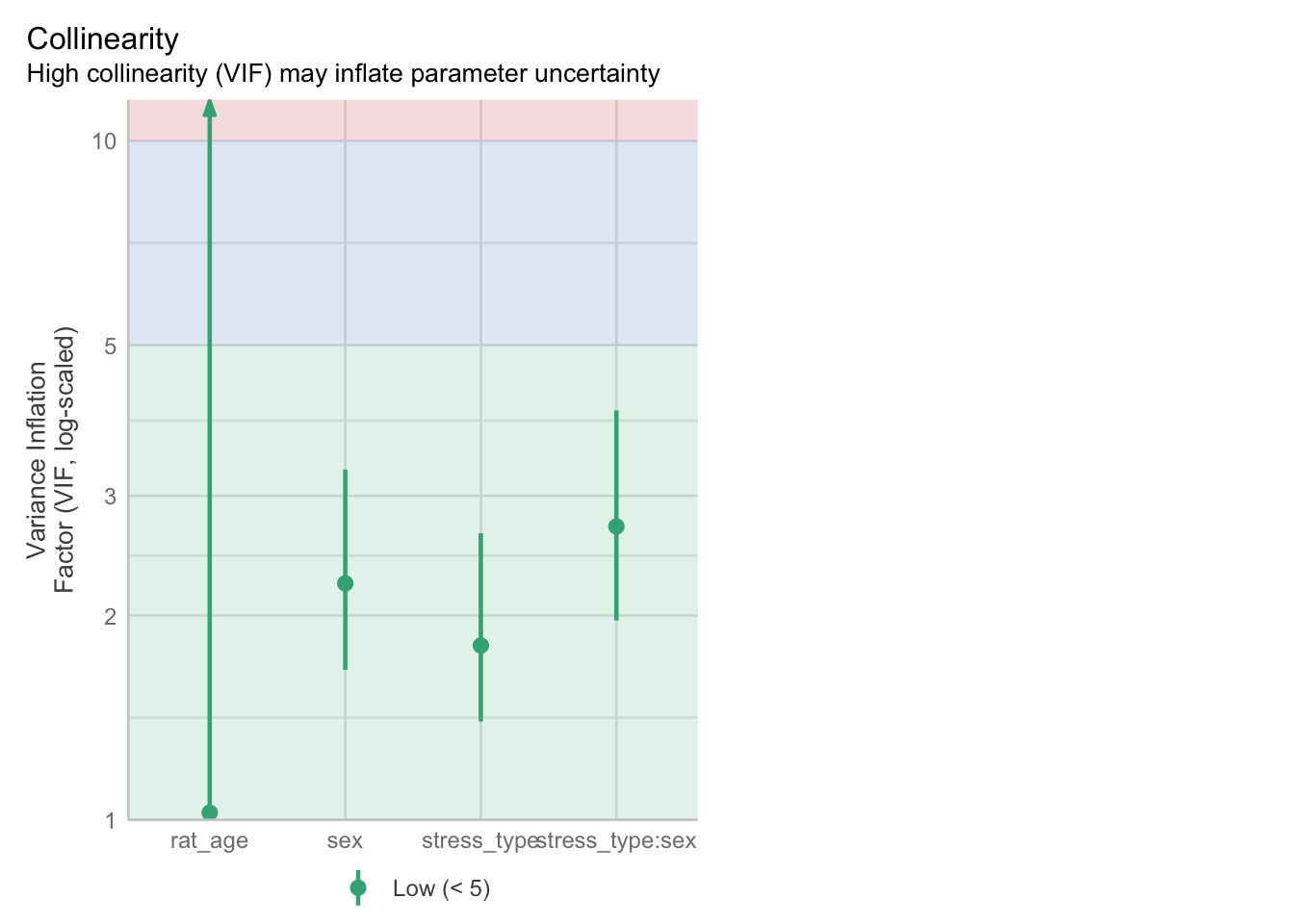

Remember to drop the response variables (and also rat ID in this case).

# Drop the response variable
X = levers.drop(columns=['rat_id','correct_presses','prop_correct','incorrect_presses'])

# Create design matrix
X = dmatrix("stress_type * sex + rat_age", data=levers, return_type='dataframe')

# Calculate VIF for each feature
vif_data = pd.DataFrame()
vif_data['feature'] = X.columns
vif_data['VIF'] = [variance_inflation_factor(X.values, i)
                   for i in range(X.shape[1])]

print(vif_data)

                               feature        VIF
0                            Intercept  48.157694
1              stress_type[T.stressed]   1.768004
2                          sex[T.male]   2.190167
3  stress_type[T.stressed]:sex[T.male]   2.799690
4                              rat_age   1.016442

Again, all good - none of our predictors have a concerning VIF.

Collectively, it would seem that our model does indeed meet the assumptions, and there are no glaring obstacles to us proceeding with a significance test and an interpretation.

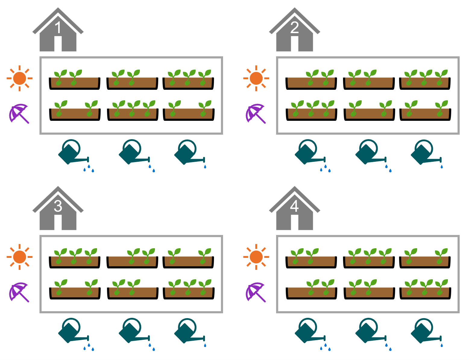
11.6.2 Seed germination

Exercise 2 - Seed germination

Level:

This exercise uses a new dataset, seeds, which is all about a seed germination experiment.

Each row of the dataset represents a seed tray, in which 25 seeds were planted. The trays were treated with one of two light conditions (sun, shade) and one of three watering frequencies (low, medium, high).

The researchers want to know whether either or both of these predictors have an affect on the proportion of seeds that successfully germinate.

In this exercise, you should:

Visualise the data
Fit a suitable model
Test the assumptions and quality of model fit
Decide whether to draw a biological conclusion from the data

R
Python

seeds <- read_csv("data/seeds.csv")

seeds = pd.read_csv("data/seeds.csv")

There is no formal worked answer provided. However, all of the code you will need can be adapted from the diabetes and aphids examples worked through in the chapter.

You are also strongly encouraged to work with, or share your answer with, a neighbour.

Hints

Consider a possible interaction effect
Look closely at the dataset itself, and all its columns
You should find at least two issues and/or failures of assumptions!

It may help to visualise the experimental design (the number of trays has been simplified so that the figure fits on the page):

11.7 Summary

While generalised linear models make fewer assumptions than standard linear models, we do still expect certain things to be true about the model and our variables for GLMs to be valid.

Key points

For a generalised linear model, we assume that we have chosen the correct link function, that our response variable follows a distribution from the exponential family, and that our data are independent
We also want to check that there are no overly influential points, no collinearity, and that the dispersion parameter is close to 1
To assess some of these assumptions/qualities, we have to rely on our understanding of our dataset
For others, we can calculate metrics like Cook’s distance and variance inflation factor, or produce diagnostic plots