9 tSNE
TipLearning Objectives
- Bulleted list of learning objectives
- Why PCA does not work sometimes
- The intution around the curse of dimensionality
- What is tSNE?
- How to use tSNE
9.1 The curse of dimensionality
In very high-dimensional spaces, almost all the “volume” of a dataset lives near its corners, and pairwise Euclidean distances between points tend to concentrate around a single value.
9.2 Simplified explanations
Think of each cell as a point in a space where each gene’s activity is its own “axis.” When you have only a few genes (low dimensions), you can tell cells apart by how far apart they sit in that space. But as you add more genes, almost every cell ends up about the same distance from every other cell—so you lose any useful sense of “close” or “far.”
Imagine you’re trying to find similar cells in a dataset. As you measure more features (dimensions), it becomes harder to find truly similar cells, even though you have more information.
9.3 Visual Example: Finding Similar Points
9.3.1 1 Dimension (1 feature)
Feature 1: [0]----[1]----[2]----[3]----[4]----[5]
           A      B      C      D      E      F

Points A and B are close (distance = 1)
Points A and F are far (distance = 5)
9.3.2 2 Dimensions (2 features)
Feature 2: 5 |     F
           4 |  E
           3 |     D
           2 |  C
           1 |     B
           0 |A
             0  1  2  3  4  5  Feature 1

Points A and B are still close
Points A and F are still far
9.3.3 3+ Dimensions (3+ features)
Feature 3: 5 |     F
           4 |  E
           3 |     D
           2 |  C
           1 |     B
           0 |A
             0  1  2  3  4  5  Feature 1

Feature 4, 5, 6... (more dimensions)

As dimensions increase:
- All points become equally distant from each other
- "Close" and "far" lose meaning
- Finding similar cells becomes impossible
9.4 Why This Happens: The “Empty Space” Problem
2D Circle - most area near the edge:
    ████████
  ██••••••██
 ██••••••••██
██••••••••••██
██••••••••••██
 ██••••••••██
  ██••••••██
    ████████
Tip
NOTE (IMPORTANT CONCEPT):
ALL volume concentrates at the “surface” The interior becomes essentially EMPTY!
Your data points all end up at the edges, far apart from each other.
9.5 High-dimensions are counter-intuitive
Counter-intuitive things happen in high dimensions. For example, most of the volume is near the edges!
Why k-Means fails:
k-Means tries to draw boundaries around groups by asking “Which centroid (group center) is each cell closest to?” In very high–gene spaces, every cell is nearly the same distance from all centroids. Small moves of the centroids don’t change which cells get assigned to them, so k-Means can’t find real groupings.
Why t-SNE helps:
t-SNE ignores the idea of absolute distance and instead asks, “Which cells are each cell’s few nearest neighbors?” It builds a map that keeps those local neighborhoods intact. In the final 2D picture, cells that were neighbors in the huge gene space stay neighbors on the screen, while cells that weren’t neighbors get pushed apart. This way, you still see meaningful clusters (e.g., cell types) even when dealing with hundreds or thousands of genes.
9.6 TLDR (Simple explanation)
t-SNE (pronounced “tee-snee”) is a tool that helps us look at complex data by making it easier to see patterns.
9.6.1 Imagine this:
- You have a big box of mixed beads. Each bead has many features: color, size, shape, weight, etc.
- It is hard to see how the beads are similar or different just by looking at all these features at once.
9.6.2 What t-SNE does:
- t-SNE takes all those features and creates a simple map (like a 2D picture).
- In this map, beads that are similar to each other are placed close together.
- Beads that are very different are placed far apart.
9.7 Pictorial explanation of tSNE
High-dimensional beads (hard to see groups):
[🔴] [🔵] [🟢] [🟡] [🔴] [🟢] [🔵] [🟡] [🔴] [🟢] [🔵] [🟡]
Each bead has many features (color, size, shape, etc.)
    |
    v
t-SNE makes a simple 2D map:
[🔴] [🔴] [🔴] | | [🔵] [🔵] [🔵]
[🟢] [🟢] [🟢]
[🟡] [🟡] [🟡]
Now, similar beads are grouped together.
In summary:
t-SNE is like a magic tool that turns complicated data into a simple picture, so we can easily see groups and patterns—even if we do not understand the math behind it!
9.7.1 Why is this useful?
- It helps us see groups or clusters in our data.
- We can spot patterns, like which beads are most alike, or if there are outliers.
- Emphasis on preserving local structure.
9.8 Why t‑SNE Works in High Dimensions
- Bypasses global distance concentration by focusing on nearest neighbors.
TipThe complex explanation
In very high-dimensional spaces, almost all the “volume” of a dataset lives near its corners, and pairwise Euclidean distances between points tend to concentrate around a single value. As dimension \(n\) grows, the volume of an inscribed ball in the hypercube \([-1,1]^n\) shrinks toward zero, and the ratio
\[ \frac{\max d - \min d}{\min d} \]
for distances \(d\) between random points rapidly approaches zero. Intuitively, “nearest” and “farthest” neighbors become indistinguishable, so any method that relies on global distances (like k-Means) loses its ability to meaningfully separate points into clusters.
k-Means clustering exemplifies this breakdown: it repeatedly assigns each point to its nearest centroid based on squared-distance comparisons. When all inter-point distances look almost the same, tiny shifts in centroid positions barely affect those assignments, leading to noisy labels and flat optimization landscapes with no clear gradients. In practice, k-Means can “get stuck” or fail to discover any meaningful grouping once dimensions rise into the dozens or hundreds.
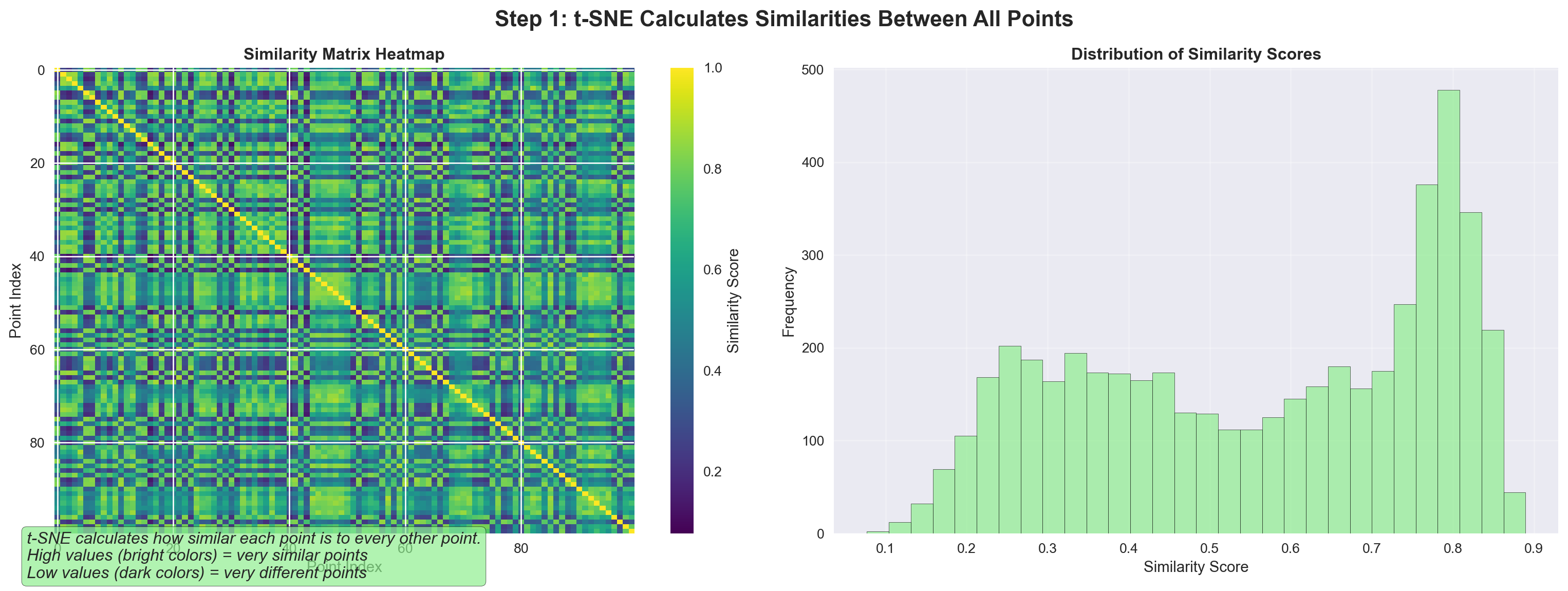
t-SNE sidesteps these problems by focusing only on local similarities rather than global distances. It first converts pairwise distances in the high-dimensional space into a distribution of affinities \(p_{ij}\) using Gaussian kernels centered on each point. Then it searches for a low-dimensional embedding whose Student-t affinity distribution \(q_{ij}\) best matches \(p_{ij}\). By emphasizing the preservation of each point’s nearest neighbors and using a heavy-tailed low-dimensional kernel to push dissimilar points apart, t-SNE highlights local clusters even when global geometry has become uninformative—making it a far more effective visualization and exploratory tool in very high dimensions.
9.9 Intuitive explanation of tSNE
9.10 Digging into tSNE
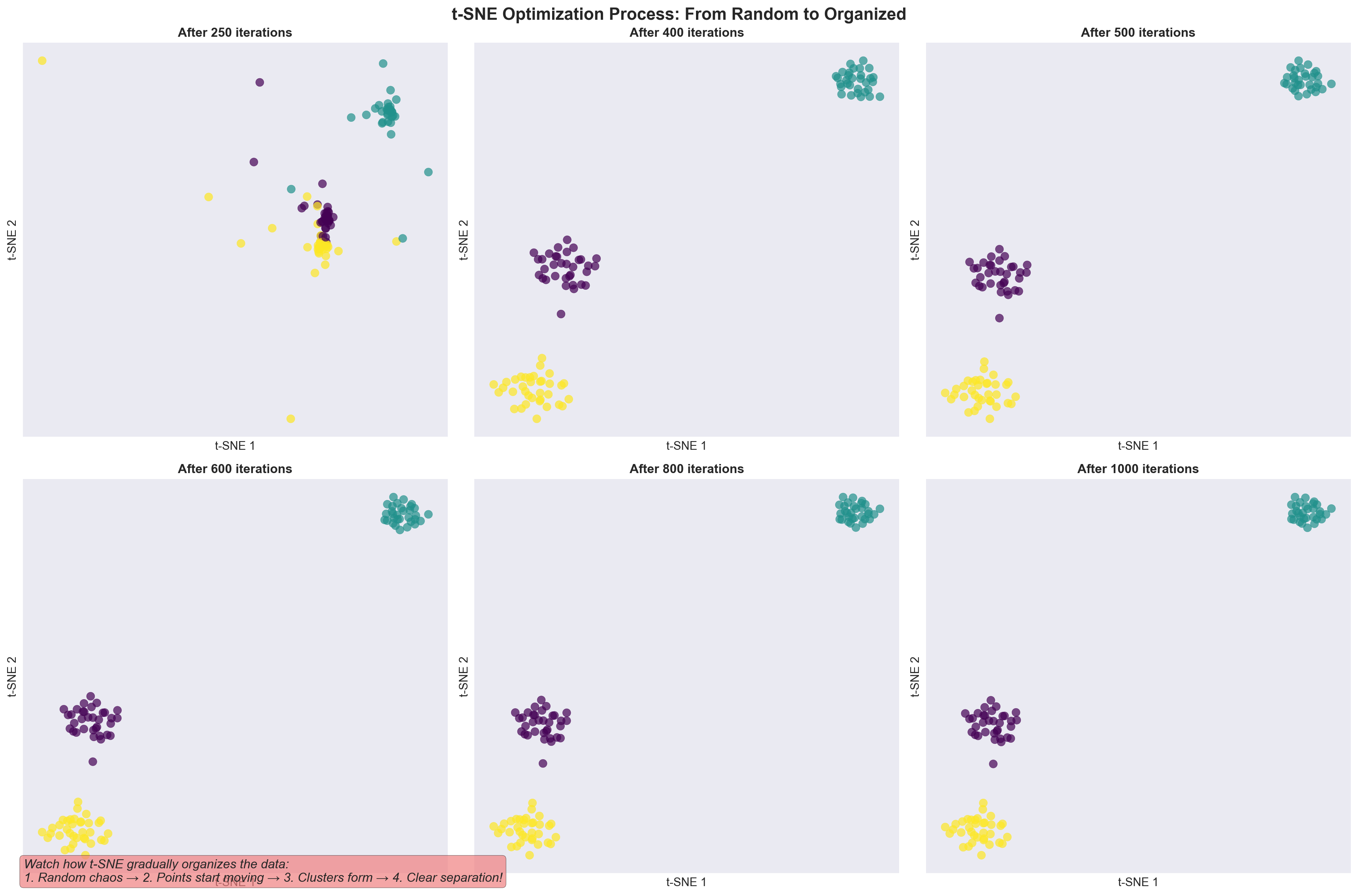
9.11 tSNE works iteratively
tSNE works iteratively to find similar points and brings them together. This is similar to clustering which we will encounter later.
tSNE gradually moves points to preserve neighborhoods. 🎯 Similar points are pulled together, different cells pushed apart.
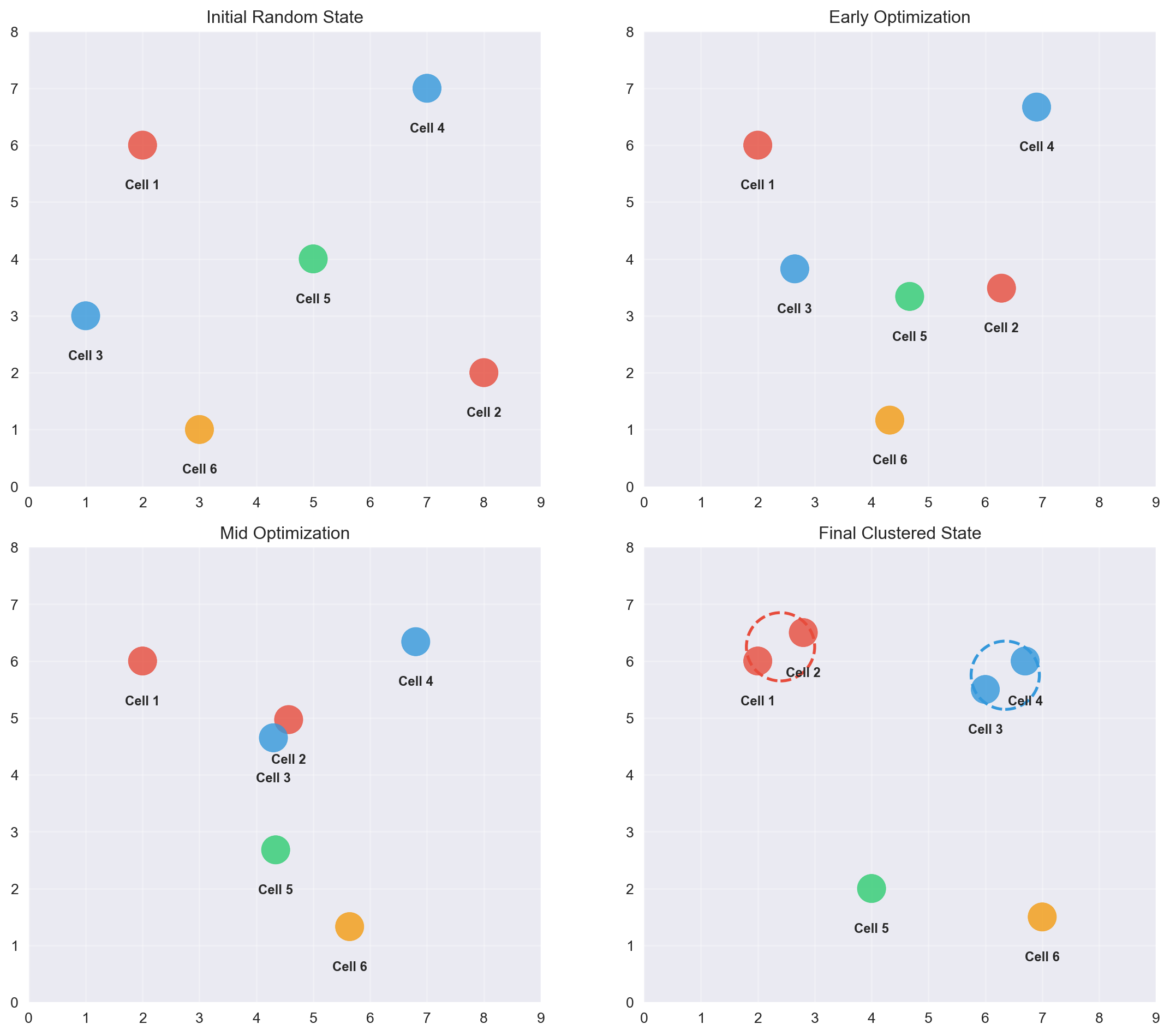
- An animation of how tSNE works
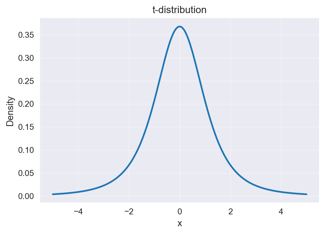
9.12 Using a t-distribution over points
Problem in 2D: When we compress high‑dimensional data into 2D, many points that were moderately far apart get squashed together. With a Gaussian in 2D, those “far” points all look similarly unlikely, which causes crowding in the center.
t-distribution has heavy tails: It decreases more slowly than a Gaussian. So points that are moderately far apart in 2D still get some probability—not zero.
What this achieves:
- Reduces crowding in the middle of the plot.
- Spreads clusters out more naturally.
- Preserves local neighborhoods (close points stay close) while allowing space between different groups.
Intuition: In high dimensions we can identify close neighbours well. In 2D there isn’t enough room, so everything would pile up. The heavy tails of the t‑distribution give extra “elbow room,” keeping clusters distinct and easier to interpret.
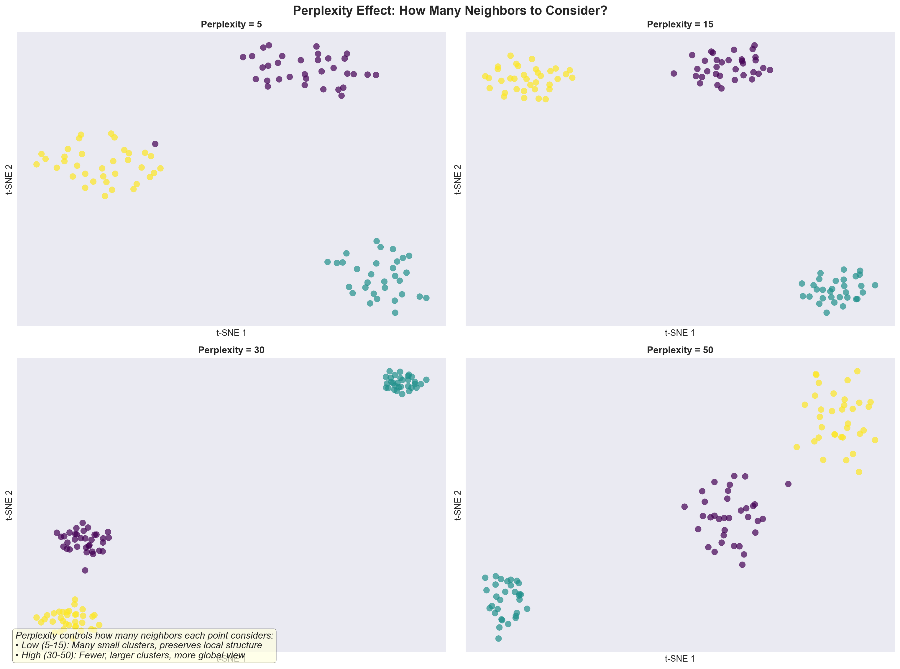
9.13 Explanation of perplexity
tSNE has an important parameter called perplexity.
What it is: Perplexity is like the number of close friends each point listens to when arranging the map.
How to think about it: It sets the typical neighborhood size.
- Low perplexity: each point cares about a small, tight circle.
- High perplexity: each point listens to more distant neighbors too.
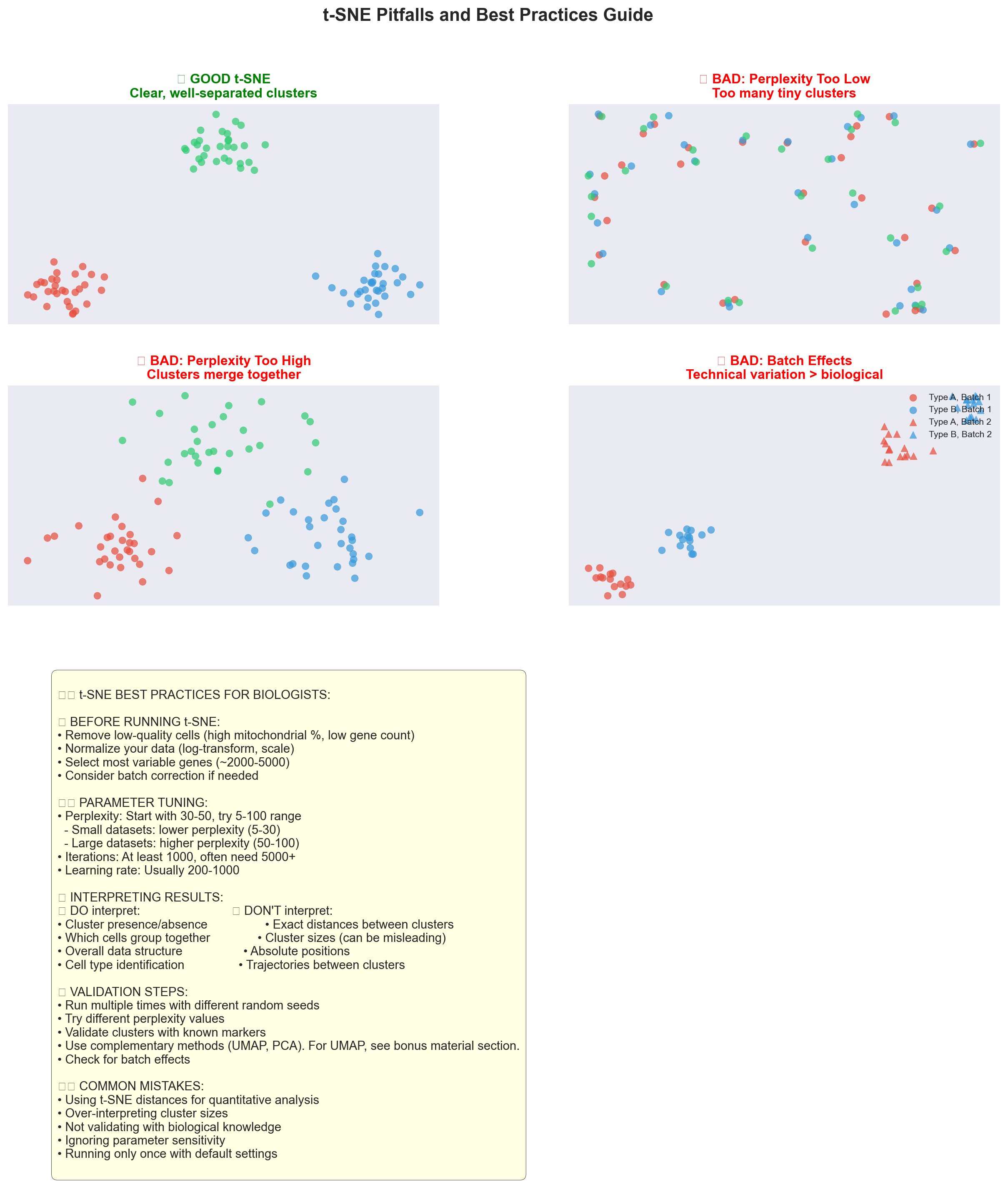
If it’s too low: You may get tiny, fragmented clusters or noisy structure.
If it’s too high: Different groups can blur together, losing fine details.
Good starting range: 5–50 (try a few values to see what’s most interpretable).
Analogy: Imagine placing cells on a 2D table. Perplexity decides how many nearby “reference cells” each one considers when finding its spot—too few and it overfits tiny patterns; too many and it smooths away meaningful differences.
9.14 How to choose perplexity?
The most appropriate value of perplexity depends on the density of your data. Loosely speaking, one could say that a larger / denser dataset requires a larger perplexity. Typical values for the perplexity range between 5 and 50.
9.15 Key Concept
TipKey Points
- Perplexity in t-SNE acts like a knob for the effective number of nearest neighbours.

9.16 Activity: Interactive figure showing tSNE and perplexity
Here is an interactive tSNE on the Swiss roll dataset (we will encounter this later). Play around with this figure and use the slider to change the value of perplexity!
9.17 Exercise: Building intuition on how to use tSNE
Let us read the paper How to use t-SNE effectively (Wattenberg, Viégas, and Johnson 2017).
Distances are not preserved
Normal does not always look normal
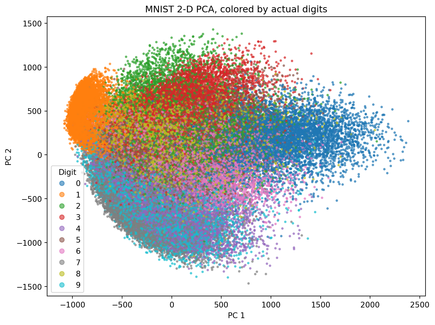
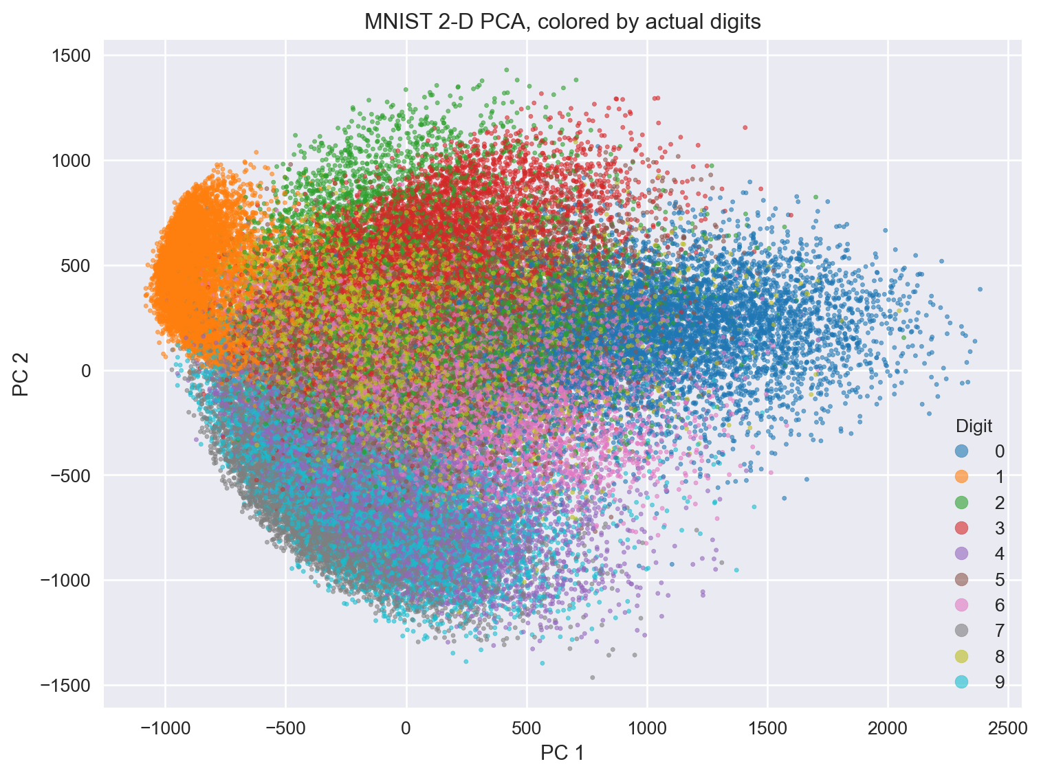
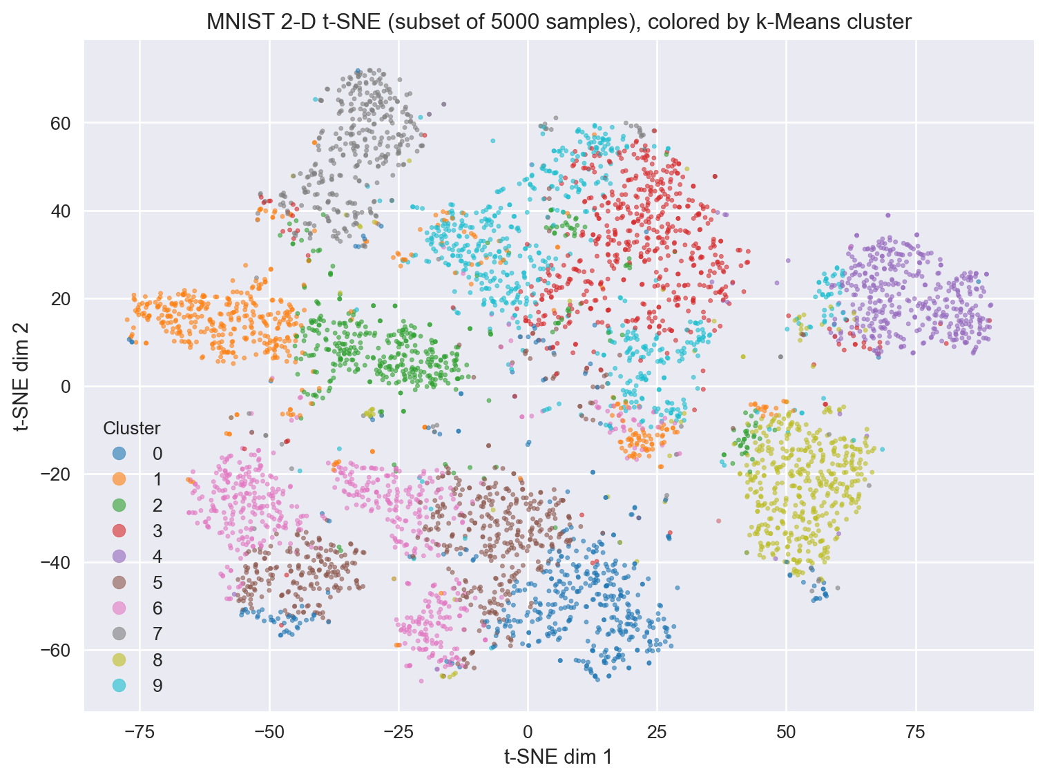
9.18 What does tSNE look like compared to PCA?
9.19 Simple code to perform tSNE (hands-on exercise)
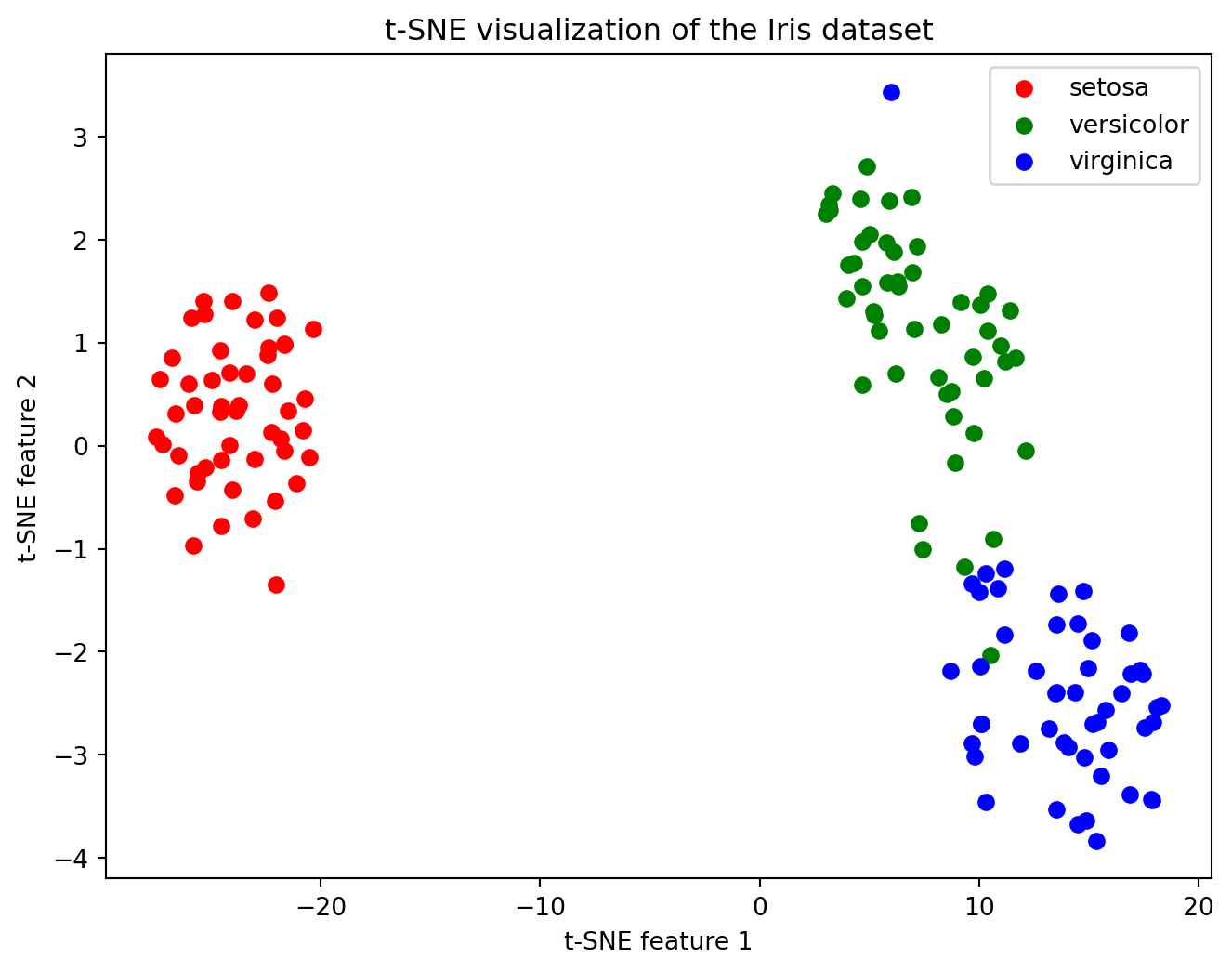
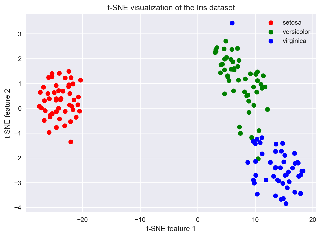
Let us now practice performing tSNE on some data. We will use the iris data. The Iris dataset is a small, classic dataset in machine learning.
It contains measurements of 150 flowers from three species of iris (setosa, versicolor, virginica).
For each flower, four features are recorded: - Sepal length - Sepal width - Petal length - Petal width
import matplotlib.pyplot as plt
from sklearn import datasets
from sklearn.manifold import TSNE
import pandas as pd

# Load the Iris dataset
iris = datasets.load_iris()
X = iris.data            # The features (measurements)
y = iris.target          # The species labels (0, 1, 2)

# create a data frame for easier viewing
df_iris_simple = pd.DataFrame(X, columns = iris.feature_names)

df_iris_simple['species'] = iris.target
df_iris_simple['species_name'] = df_iris_simple['species'].map( {0:'setosa', 1:'versicolor', 2:'virginica'} )

# display basic information
print(df_iris_simple.head)

# scatter plots
plt.figure()
plt.scatter(X[:,0], X[:,1], c = iris.target, cmap='viridis')
plt.xlabel(iris.feature_names[0])
plt.ylabel(iris.feature_names[1])
plt.title('Sepal length vs. Sepal width')
plt.colorbar(label='species')
plt.show()


# Run t-SNE to reduce the data to 2 dimensions
tsne = TSNE(n_components=2, random_state=0, perplexity=30)
X_2d = tsne.fit_transform(X)

# Plot the results (simple plot)
plt.figure()
plt.scatter(X_2d[:,0], X_2d[:,1], c = y) # color by spcies labels
plt.show()

# Plot the results, one species at a time
plt.figure()
# Setosa (label 0)
idx_y_0 = (y == 0) # get index of those flowers where y == 0
plt.scatter(X_2d[idx_y_0,0], X_2d[idx_y_0,1], color='red', label='setosa')

# Versicolor (label 1)
idx_y_1 = (y == 1) # get index of those flowers where y == 1
plt.scatter(X_2d[idx_y_1,0], X_2d[idx_y_1,1], color='green', label='versicolor')

# Virginica (label 2)
idx_y_2 = (y == 2) # get indices of when y is 2
plt.scatter(X_2d[idx_y_2,0], X_2d[idx_y_2,1], color='blue', label='virginica')

plt.xlabel("t-SNE feature 1")
plt.ylabel("t-SNE feature 2")
plt.title("t-SNE visualization of the Iris dataset")
plt.legend()
plt.show()
<bound method NDFrame.head of sepal length (cm) sepal width (cm) petal length (cm) petal width (cm) \
0 5.1 3.5 1.4 0.2
1 4.9 3.0 1.4 0.2
2 4.7 3.2 1.3 0.2
3 4.6 3.1 1.5 0.2
4 5.0 3.6 1.4 0.2
.. ... ... ... ...
145 6.7 3.0 5.2 2.3
146 6.3 2.5 5.0 1.9
147 6.5 3.0 5.2 2.0
148 6.2 3.4 5.4 2.3
149 5.9 3.0 5.1 1.8
species species_name
0 0 setosa
1 0 setosa
2 0 setosa
3 0 setosa
4 0 setosa
.. ... ...
145 2 virginica
146 2 virginica
147 2 virginica
148 2 virginica
149 2 virginica
[150 rows x 6 columns]>
9.20 Exercise: tSNE is stochastic
Stochasticity: play around with the
random_stateparameter. Does your tSNE plot look different to the person you are seated next to?Play around with the
perplexityparameter (pair up with someone)Which value of
perplexityshould you use?
9.21 Key Concept
TipKey Points
- Recall that unsupervised machine learning can help you come up with new hypotheses
- Vary the perplexity parameter: ideally your patterns or hypotheses should be true even if you change perplexity
9.22 Perplexity pitfalls and things to watch out for
9.23 Exercise: Hands-on practical applying tSNE to another dataset
Work in a group.
Load the US Arrests data in Python and perform tSNE on this (pair up with a person)
Some code to help you get started is here:
import pandas as pd
import matplotlib.pyplot as plt
from sklearn.manifold import TSNE

# Load the US Arrests data
url = "https://raw.githubusercontent.com/cambiotraining/ml-unsupervised/main/course_files/data/USArrests.csv"
df = pd.read_csv(url, index_col=0)

# Prepare the data for t-SNE
X = df.values

# Fill in your code here ..........
How would you evaluate this?
Vary the
perplexityparameter
Also annotate the plot by US states. Hint: Use the
plt.annotate()function. The US states names are available indf.index.Is
Californiastill far apart fromVermonteven if you change theperplexityparameter?
9.24 Other algorithms
We have given a brief overview of some unsupervised machine learning techniques. There are many others. For example, you can also read about UMAP
9.25 Summary
TipKey Points
- High dimensions make global distances meaningless.
- Methods that leverage local structure (t‑SNE) can still find patterns.
- tSNE is stochastic and can be hard to interpret
- Vary the
perplexityparameter (ideally your patterns or hypotheses should be true even if you change perplexity)
9.26 References
[1] How to Use t-SNE Effectively