!pip install pandas numpy scikit-learn seaborn matplotlib scanpy pca5 Refresher on Python
TipLearning Objectives
- Refresher on Python
5.1 Refresher on Python
See Python setup instructions here: Python Installation.
Walkthrough of getting setup with Google Colab in the web browser.
Install Python packages
- Loading data and data visualization
Note: Here is an alternative way to read a file
import pandas as pd
import os
# find out which directory is your current working directory
os.getcwd()
# now change directory to where your files are (my files are in the directory shown below)
os.chdir("/Users/soumyabanerjee/soumya_cam_mac/teaching/ml-unsupervised/")
# now read the file
diabates_data = pd.read_csv("course_files/data/diabetes_sample_data.csv")
# 1. IMPORTING PACKAGES
import pandas as pd
import matplotlib.pyplot as plt
import numpy as np
import os
# 2. READING DATA WITH PANDAS FROM GITHUB
# GitHub URL for the diabetes data
# Convert from GitHub web URL to raw data URL
github_url = "https://raw.githubusercontent.com/cambiotraining/ml-unsupervised/main/course_files/data/diabetes_sample_data.csv"
# Read CSV file directly from GitHub
diabetes_data = pd.read_csv(github_url)
# Display basic information about the data
print("\nData shape:", diabetes_data.shape)
print("\nFirst 5 rows:")
print(diabetes_data.head())
print("\nBasic statistics:")
print(diabetes_data.describe())
# 3. PLOTTING WITH MATPLOTLIB
# Plot 1: Histogram of Age
plt.figure()
plt.hist(diabetes_data['age'], bins=20, alpha=0.7)
plt.title('Distribution of Age', fontsize=14, fontweight='bold')
plt.xlabel('Age')
plt.ylabel('Frequency')
plt.grid(True, alpha=0.3)
plt.savefig('age_distribution.png', dpi=300)
plt.show()
# 4. NUMPY
a = np.array([17, 13, 78, 901])
print("This is a numpy array:")
print(a)
print("Here is the mean/average:")
print( np.mean(a) )
Data shape: (100, 6)

First 5 rows:
   patient_id   age  glucose   bmi  blood_pressure  diabetes
0           1  62.5     97.5  29.8            71.7         0
1           2  52.9    127.4  30.8            74.4         0
2           3  64.7    129.7  33.4            87.5         0
3           4  77.8    115.9  33.3            86.1         1
4           5  51.5    135.2  21.1            79.8         1

Basic statistics:
       patient_id         age     glucose         bmi  blood_pressure  \
count  100.000000  100.000000  100.000000  100.000000      100.000000
mean    50.500000   53.444000  140.670000   28.322000       81.066000
std     29.011492   13.625024   28.611669    5.425223        8.842531
min      1.000000   15.700000   82.400000   11.800000       58.800000
25%     25.750000   46.000000  115.800000   24.700000       74.350000
50%     50.500000   53.100000  142.550000   28.500000       80.500000
75%     75.250000   61.075000  156.175000   31.500000       86.825000
max    100.000000   82.800000  221.600000   47.300000      101.900000

         diabetes
count  100.000000
mean     0.250000
std      0.435194
min      0.000000
25%      0.000000
50%      0.000000
75%      0.250000
max 1.000000 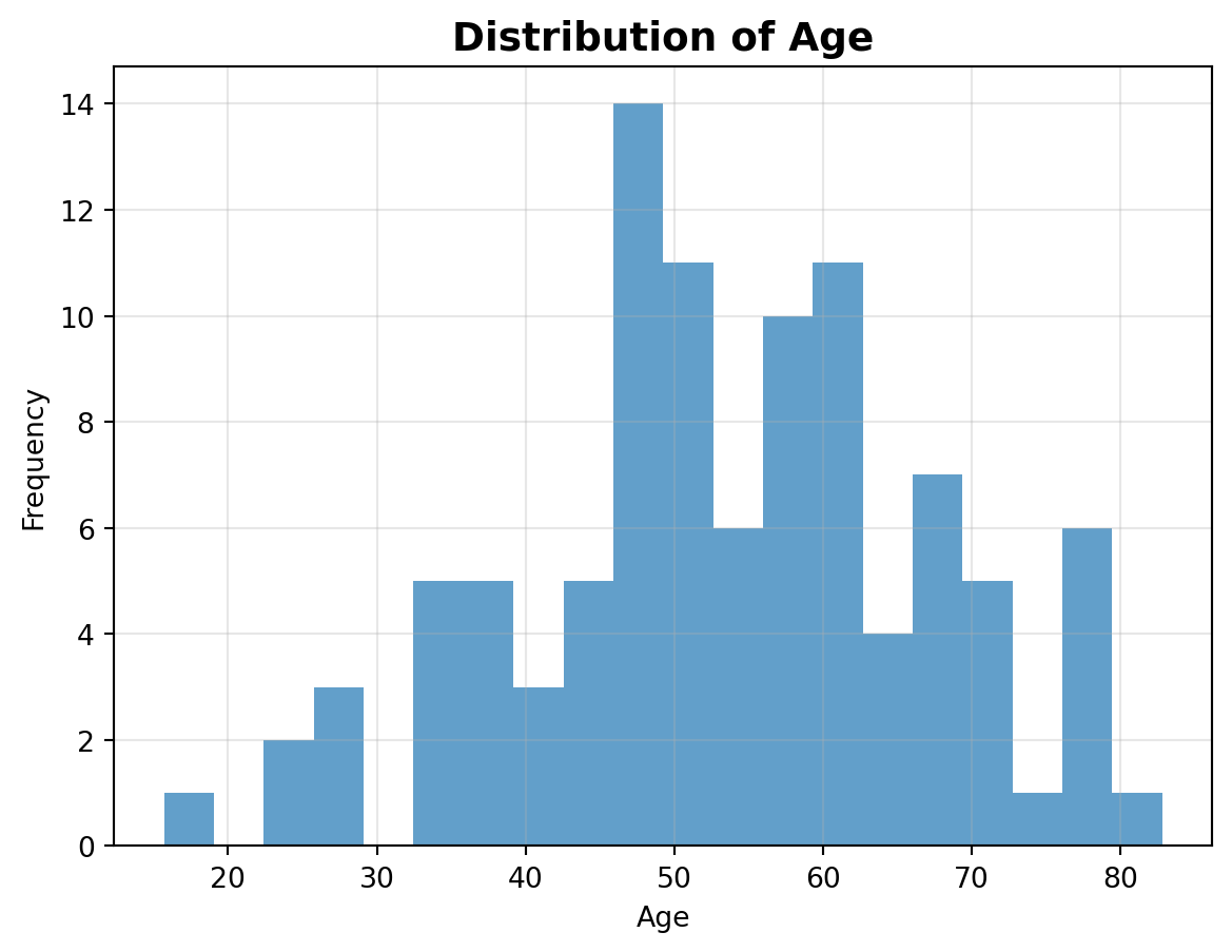
This is a numpy array:
[ 17  13  78 901]
Here is the mean/average:
252.25- You can also go through this Introduction to Visualization in Python course
5.1.1 Optional exercise on Python
5.1.2 Optional exercise on Python
ExerciseExercise 2 - exercise_python_visualization
Level:
Load the dataset from this GitHub URL:
https://raw.githubusercontent.com/cambiotraining/ml-unsupervised/refs/heads/main/course_files/data/USArrests.csv
Histogram: Show the distribution of murders
- Use
plt.hist()with theMurdercolumn
- Use 15 bins
- Add title: “Distribution of Murder”
- Add axis labels and grid
Remember to use plt.show() after each plot!
AnswerAnswer
Simple data visualization
import pandas as pd
import matplotlib.pyplot as plt

# Load the dataset
url = "https://raw.githubusercontent.com/cambiotraining/ml-unsupervised/refs/heads/main/course_files/data/USArrests.csv"
crime_data = pd.read_csv(url)

# Draw histogram
plt.figure()
plt.hist(crime_data["Murder"], bins=15)
plt.grid(True)
plt.xlabel("Murder")
plt.ylabel("Frequency")
plt.title("Distribution of Murder")
plt.show()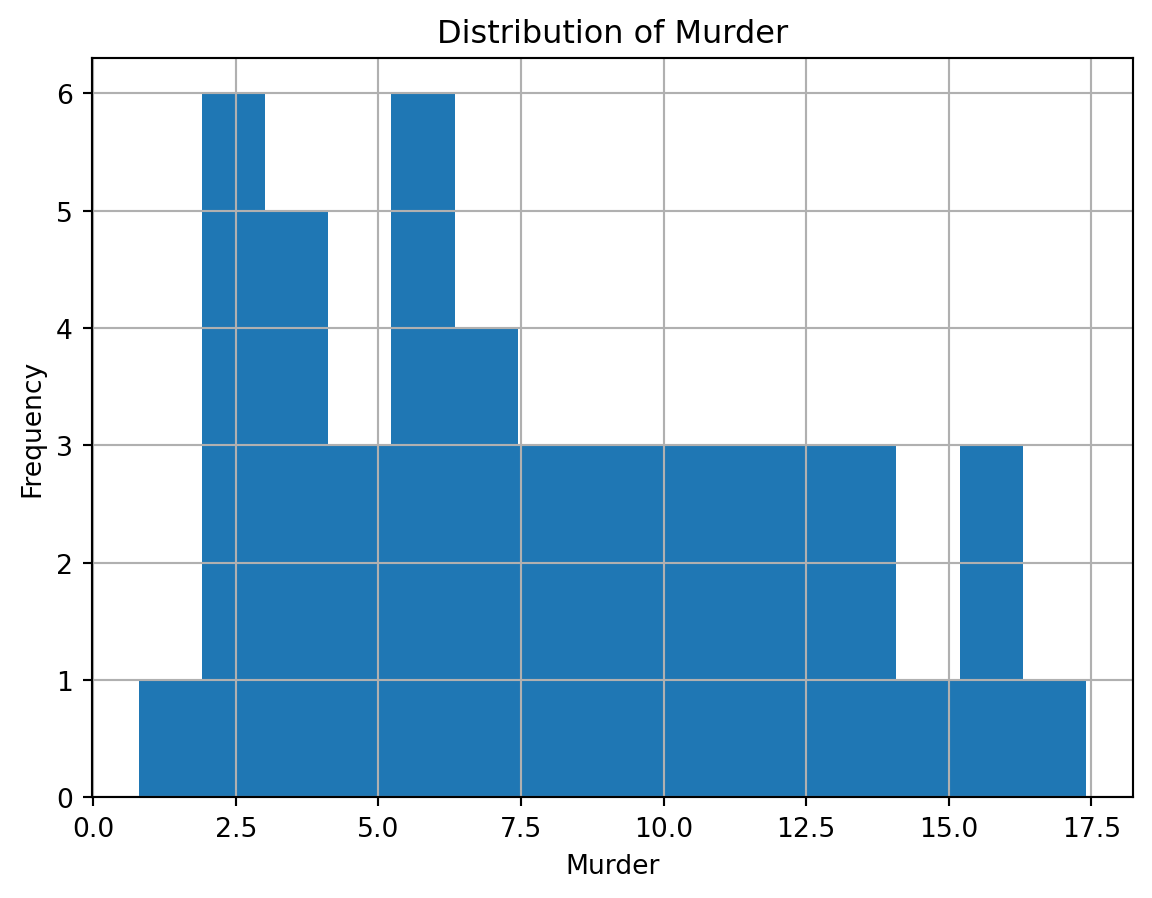
5.1.3 Optional exercise on Python
5.1.4 Optional exercise on Python
5.1.5 Optional exercise on Python
5.2 Summary
TipKey Points
- A quick refresher on Python
- Simple exercises (optional)
5.3 Resources
[1] Course on data analysis using Python