13 When PCA or tSNE might not work
TipLearning Objectives
- Understand real-world scenarios where unsupervised learning is applied
- Identify situations where PCA and other dimensionality reduction techniques may not be effective
13.1 When PCA or tSNE may not work
- Nonlinear structure
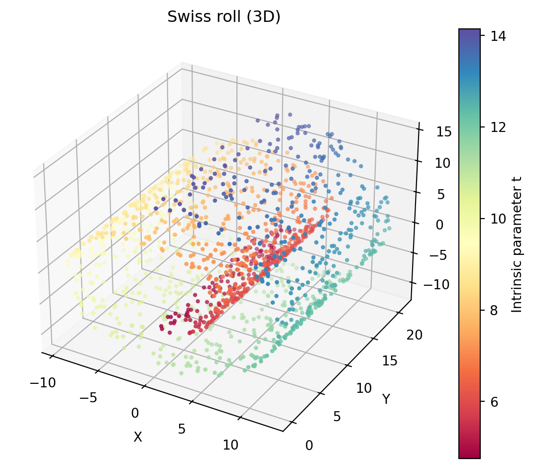
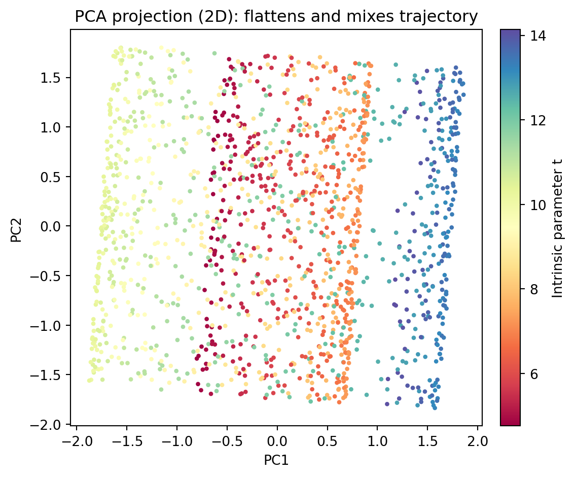
- Swiss roll/curved trajectories (e.g., differentiation trajectories); PCA flattens and mixes cells that are nearby in 2D but far along the curve.
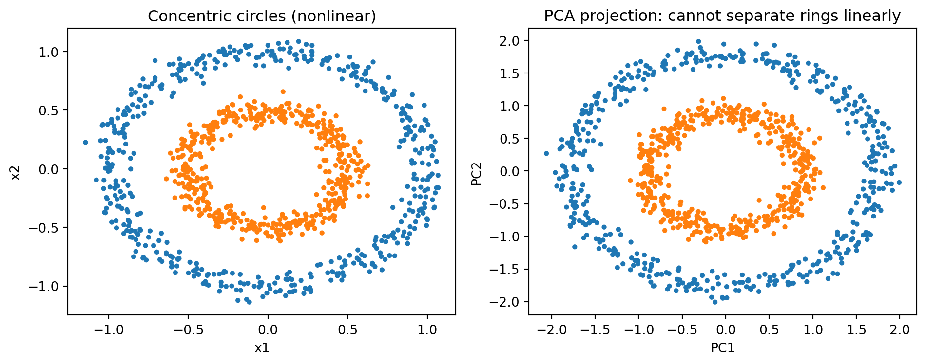
- Concentric patterns (e.g., ring-like responses); PCA cannot separate circles.
- When variance ≠ signal
- Batch effects or library size dominate variance in scRNA‑seq; PCs reflect technical factors rather than biology.
- Cell cycle effects overshadow subtle lineage differences.
- Rare cell types: biologically important but low variance, thus missed by top PCs.
- Outliers and heavy tails
- A few extreme samples/genes drive the first PCs, masking true structure (common with QC issues or outlier libraries).
- Feature scaling and units
- Mixed units or unscaled features: high-variance genes/proteins dominate; low-variance but important markers get ignored.
- Time/phase structure
- Periodic processes (cell cycle phases): PCA captures amplitude rather than phase, mixing states.
- p >> n instability
- Many more genes than samples: PCs become noisy/unstable without regularization or careful preprocessing.
- Missing data
- Nonrandom missingness (dropouts in scRNA‑seq) biases covariance; naive imputation can create artificial PCs.
13.1.1 Quick remedies
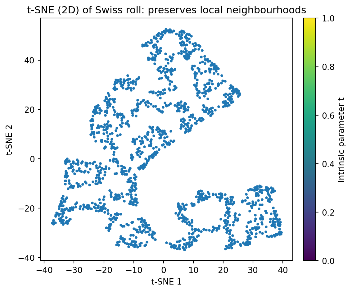
- Nonlinear structure: t‑SNE/UMAP.
- Variance ≠ signal: regress out batch/cell cycle; use sctransform; combat/BBKNN/Harmony for batch correction; consider supervised methods (PLS/CCA) if labels exist.
- Outliers/heavy tails: robust PCA, rank genes with robust dispersion, Winsorize/log1p.
- Scaling/units: standardize features; use variance-stabilizing transforms (log1p, VST).
13.1.2 Non-linear data
- Non-linearity: Data that lies on curved surfaces or when data has non-linear relationships.
- Single-cell data: Biological data where cell types form non-linear clusters in high-dimensional space
13.1.3 Categorical Features
- PCA may work poorly with categorical data unless properly encoded
- One-hot encoding categorical features can create sparse, high-dimensional data where PCA may not capture meaningful structure
13.2 Alternatives
13.2.1 t-SNE (t-Distributed Stochastic Neighbor Embedding)
- Best for: Non-linear dimensionality reduction and visualization
- Key parameter: Perplexity (try values 5-50)
- Use case: Single-cell data, biological expression data, any non-linear clustering
Tip
NOTE (IMPORTANT CONCEPT): Sometimes tSNE may not work as well! It is hard to predict which unsupervised machine learning technique will work best.
You just need to try a bunch of different techniques.
13.2.2 Hierarchical Clustering + Heatmaps
- Best for: Categorical data and understanding relationships between samples
- Use case: When you want to see how samples group together based on multiple features
13.2.3 Activity: Demonstrating how PCA may not work well on the Swiss roll data
- The
Swiss rolldataset
A 2D curve embedded in 3D that looks like a rolled sheet. You can play around with the plot below!
- Performing PCA on the Swiss roll dataset
- Performing tSNE on the Swiss roll dataset
13.2.4 PCA on time series data and spiral data
--- TIMESERIES DATA ---PCA Analysis for Timeseries Data
==================================================
PC1 explains 69.6% of variance
PC2 explains 30.4% of variance
Total variance explained: 100.0%
Why PCA fails here:
• This is actually a function y = f(t) where t is time
• PCA treats it as 2D spatial data, ignoring temporal structure
• The relationship is nonlinear (sine waves)
• Important frequency components are lost in projection
Better alternatives:
• Manifold learning: t-SNE, UMAP, Isomap
• Kernel PCA for nonlinear relationships
• Autoencoders for complex nonlinear dimensionality reduction
• For time series: Fourier analysis, wavelet transforms
• Recurrent neural networks for temporal patterns
============================================================
--- SPIRAL DATA ---PCA Analysis for Spiral Data
==================================================
PC1 explains 54.6% of variance
PC2 explains 45.4% of variance
Total variance explained: 100.0%
Why PCA fails here:
• Data follows a spiral pattern with rotational structure
• PCA cannot capture circular/rotational relationships
• Sequential ordering (temporal aspect) is lost
• Linear projection destroys the spiral geometry
Better alternatives:
• Manifold learning: t-SNE, UMAP, Isomap
• Kernel PCA for nonlinear relationships
• Autoencoders for complex nonlinear dimensionality reduction
============================================================13.2.5 Missing data
PCA and tSNE also do not work well when there is missing data. See Exercise Section 11.1.
13.2.6 Demonstrating how PCA or tSNE may not work well on biological data
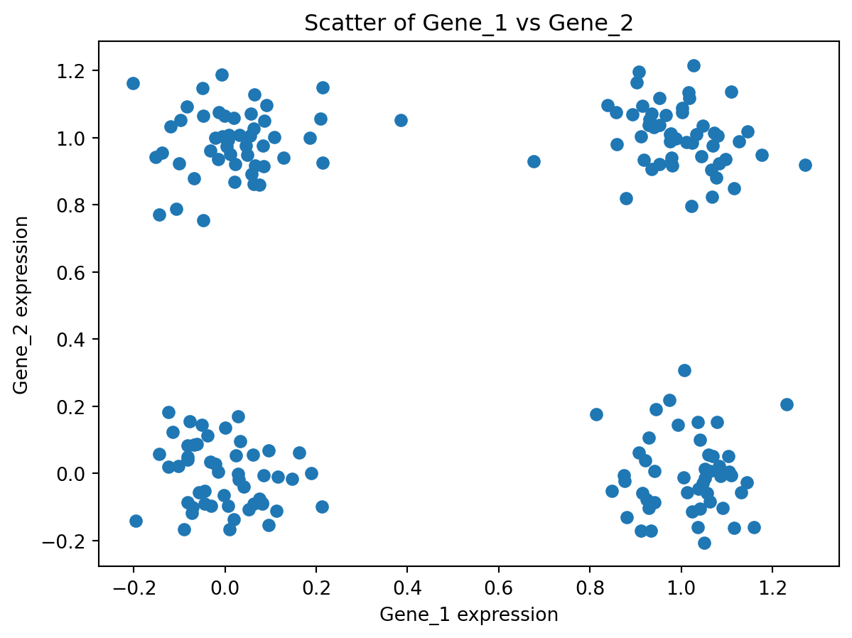
- Generate synthetic biological expression data: matrix of 200 samples × 10 genes, where Gene_1 and Gene_2 follow a clustering (four corner clusters) and the remaining genes are just Gaussian noise. You can see from the scatter of Gene_1 vs Gene_2 that the true structure is non-linear and not aligned with any single variance direction: PCA (or tSNE) may fail to unfold these clusters into separate principal components.
- Perform PCA on this data
from sklearn.decomposition import PCA
import matplotlib.pyplot as plt

# Apply PCA
pca = PCA()
pcs = pca.fit_transform(df) # where df is a dataframe with your data


# Scatter plot of the first two principal components
plt.figure()
plt.scatter(pcs[:, 0], pcs[:, 1])
plt.xlabel('PC1')
plt.ylabel('PC2')
plt.title('PCA on Synthetic Biological Dataset')
plt.show()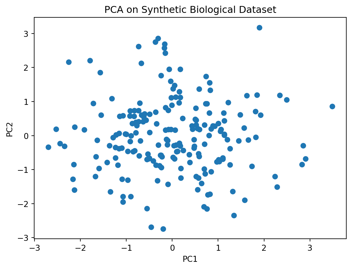
- Let us try tSNE on this data
from sklearn.manifold import TSNE
import matplotlib.pyplot as plt

tsne = TSNE()
tsne_results = tsne.fit_transform(df)

# plot
plt.figure()
plt.scatter(tsne_results[:,0], tsne_results[:,1])
plt.xlabel('t-SNE component 1')
plt.ylabel('t-SNE component 2')
plt.title('t-SNE on Synthetic Biological Dataset')
plt.show()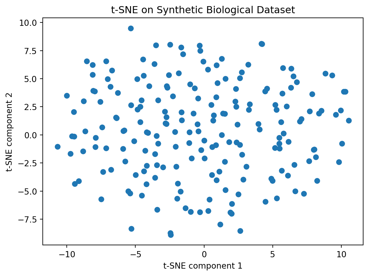
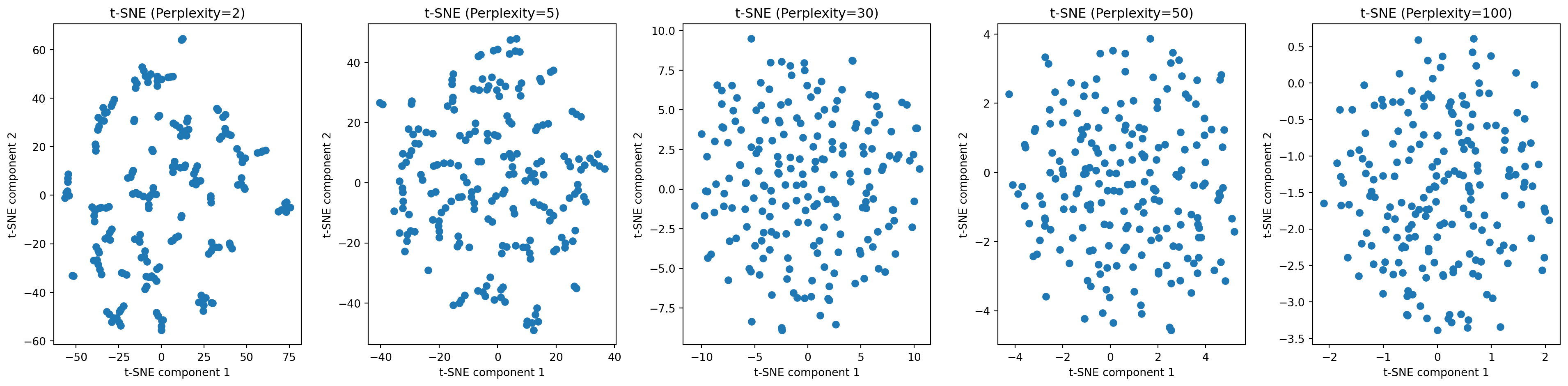
- What if we try different values of perplexity?
What if data has categorical features?
- PCA may or may not work if you have categorical features.
For example, if you have data that looks like this ….
  species tissue condition
0   human  liver  diseased
1   mouse  brain  diseased
2   human  liver  diseased
3   human  brain  diseased
4   mouse  brain   healthy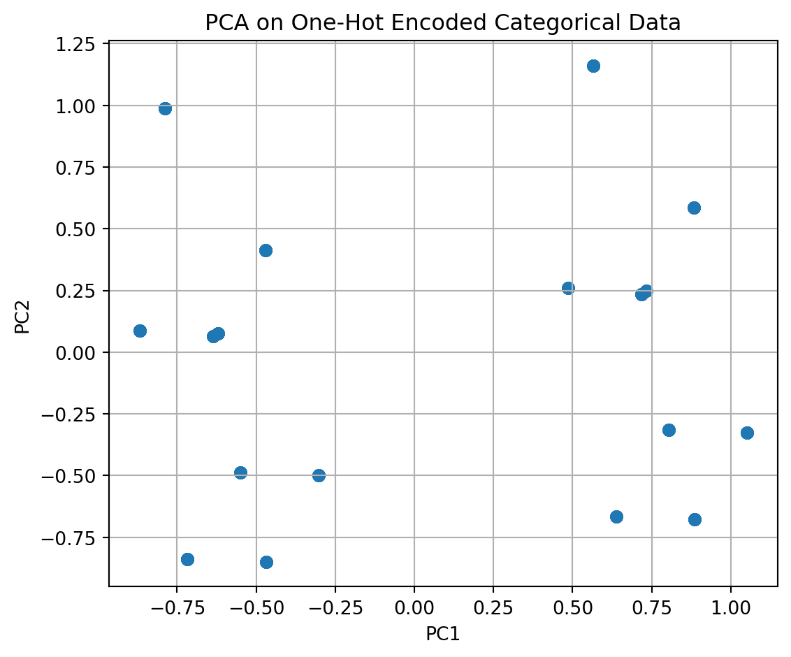
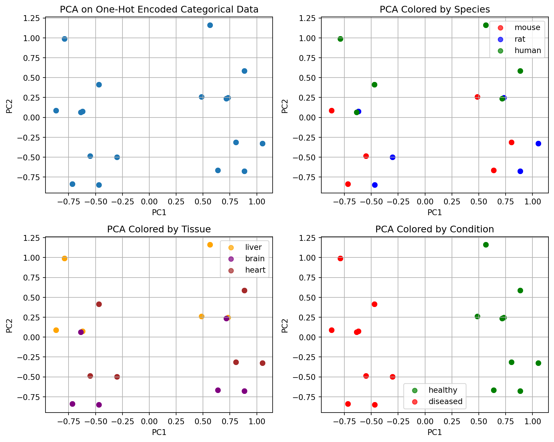
- We can split by disease/healthy, or other features.
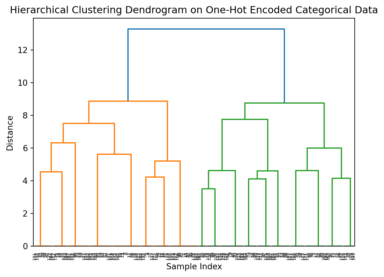
- Hierarchical clustering
Recall:
Leaves: Each leaf at the bottom of the dendrogram represents one sample from your dataset.
Branches: The branches connect the samples and groups of samples. The height of the branch represents the distance (dissimilarity) between the clusters being merged.
Height of Merges: Taller branches indicate that the clusters being merged are more dissimilar, while shorter branches indicate more similar clusters.
Clusters: By drawing a horizontal line across the dendrogram at a certain distance, you can define clusters. All samples below that line that are connected by branches form a cluster.
In the context of your one-hot encoded categorical data (species, tissue, condition), the dendrogram shows how samples are grouped based on their combinations of these categorical features.
Samples with the same or very similar combinations of categories will be closer together in the dendrogram and merge at lower distances.
The structure of the dendrogram reflects the relationships and similarities between the different combinations of species, tissue, and condition present in your synthetic dataset.
from scipy.cluster.hierarchy import dendrogram, linkage
from matplotlib import pyplot as plt
import seaborn as sns

# Assume 'encoded_data' exists from the previous one-hot encoding step
linked = linkage(y = encoded_data,
    method = 'ward',
    metric = 'euclidean',
    optimal_ordering=True
    )

# plot dendrogram
plt.figure()
dendrogram(linked,
            orientation='top',
            distance_sort='descending',
            show_leaf_counts=True)
plt.title('Hierarchical Clustering Dendrogram on One-Hot Encoded Categorical Data')
plt.xlabel('Sample Index')
plt.ylabel('Distance')
plt.show()

# or use sns.clustermap()
sns.clustermap(data=encoded_data,
method = "ward",
metric = "euclidean",
row_cluster = True,
col_cluster = True,
cmap = "vlag"
)
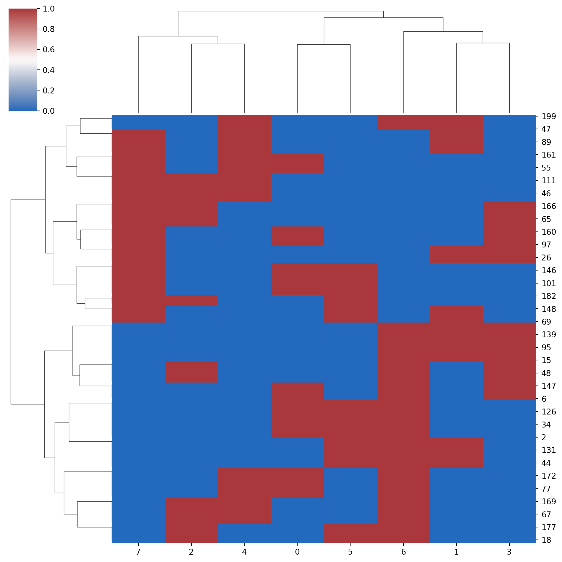
- Heatmaps
Heatmaps are a great way to visualize data and clustering
import seaborn as sns
import matplotlib.pyplot as plt

# Assume 'encoded_df' exists from the previous one-hot encoding step

plt.figure()
sns.heatmap(encoded_df.T, cmap='viridis', cbar_kws={'label': 'Encoded Value (0 or 1)'}) # Transpose for features on y-axis

plt.title('Heatmap of One-Hot Encoded Categorical Data')
plt.xlabel('Sample Index')
plt.ylabel('Encoded Feature')
plt.tight_layout()
plt.show()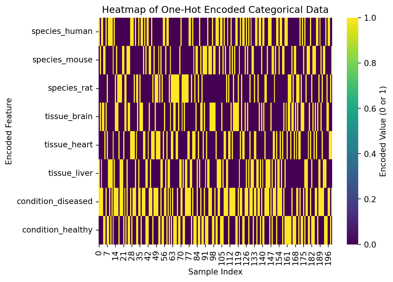
13.3 Summary
TipKey Points
- PCA or tSNE are not magic bullets and may not work all the time
- Usually you need to try a bunch of different techniques
- Remember that unsupervised machine learning is exploratory