4 Introducing random effects
Mixed effects models are particularly useful in biological and clinical sciences, where we commonly have innate clusters or groups within our datasets. This is because mixed effects models contain random effects in addition to fixed effects (hence the name, “mixed effects”).
Rather than incorrectly assuming independence between observations, random effects allow us to take into account the natural clusters or structures within datasets, without requiring us to calculate separate coefficients for each group - in other words, solving the problem of psuedoreplication, without sacrificing as much statistical power.
4.1 What is a random effect?
There are a few things that characterise a random effect:
- All random effects are categorical variables or factors
- They create clusters or groups within your dataset (i.e., non-independence)
- The levels/groups of that factor have been chosen “at random” from a larger set of possible levels/groups - this is called exchangeability
- Usually, we are not interested in the random effect as a predictor; instead, we are trying to account for it in our analysis
- We expect to have 5 or more distinct levels/groups to be able to treat a variable as a random effect
4.1.1 An example of a random effect
Let’s put the features listed above in context, with an example.
Imagine that you’re conducting a study to investigate whether temperature predicts the number of tourists that go to beaches. You study ten different beaches, and for each Saturday in the summer season that year, you record peak temperature and number of tourists.
Here, the relationship we’re interested in is number of tourists ~ peak temperature. We’ve created replicates by measuring these variables on an number of different Saturdays across the summer period. We’ve also replicated, however, by looking at 10 beaches.
This has created an additional clustering variable, and non-independence within our data: beach. Week to week, we would expect both temperature and tourists to be more similar to other values recorded on the same beach, compared to other beaches - perhaps due to factors like location, size, popularity, cleanliness and so on.
So, beach is both a categorical variable, and one that creates non-independence in our dataset.
However, we are not really interested in these specific 10 beaches. We want to know about the relationship between tourists and temperature across all beaches, ideally, and we just happen to have tested these ones. In other words, the precise beaches we tested are exchangeable with any other beaches that we might’ve investigated instead.
We want to make sure that our analysis accounts for the non-independence that the beach variable has generated, so that we can get at the actual effect of interest. Treating beach as a random effect here allows us to quantify how much of the variance in the tourists ~ temperature relationship was down to factors that are beach-specific (location and size of beach, local weather differences etc.), and how much of the variance is actually due to our overall effect of interest.
Thankfully, we estimated from 5 or more different beaches, and so we’re able to treat this variable as a random effect. Having enough levels/groups within your random effect is important for the underlying maths that goes on when you fit the model, so that you can adequately share information across the different levels.
4.2 Exercises
4.2.1 Primary schools
Level:
An education researcher is interested in the impact of socio-economic status (SES) and gender on students’ primary school achievement.
For twelve schools across the UK, she records the following variables for each child in their final year of school (age 11):
- Standardised academic test scores
- Whether the child is male or female
- Standardised SES score, based on parental income, occupation and education
The response variable in this example is the standardised academic test scores, and we have two predictors: gender and SES score. Note that we have also tested these variables across three schools.

Which of these predictors should be treated as fixed versus random effects? Are there any other “hidden” grouping variables that we should consider, based on the description of the experiment?
We care about the effects of gender and SES score. We might also be interested in testing for the interaction between them, like so: academic test scores ~ SES + gender + SES:gender.
This helps us to determine straight away that both gender and SES score are fixed effects - we’re interested in them directly. Supporting this is the fact that we have restricted gender here to a categorical variable with only two levels, while SES score is continuous - neither of these could be treated as random effects.
However, school should be treated as a random effect. We collected data from 12 different schools, but we are not particularly interested in differences between these specific schools. In fact we’d prefer to generalise our results to students across all UK primary schools, and so it makes sense to share information across the levels. But we can’t neglect school as a variable in this case, as it does create natural clusters in our dataset.
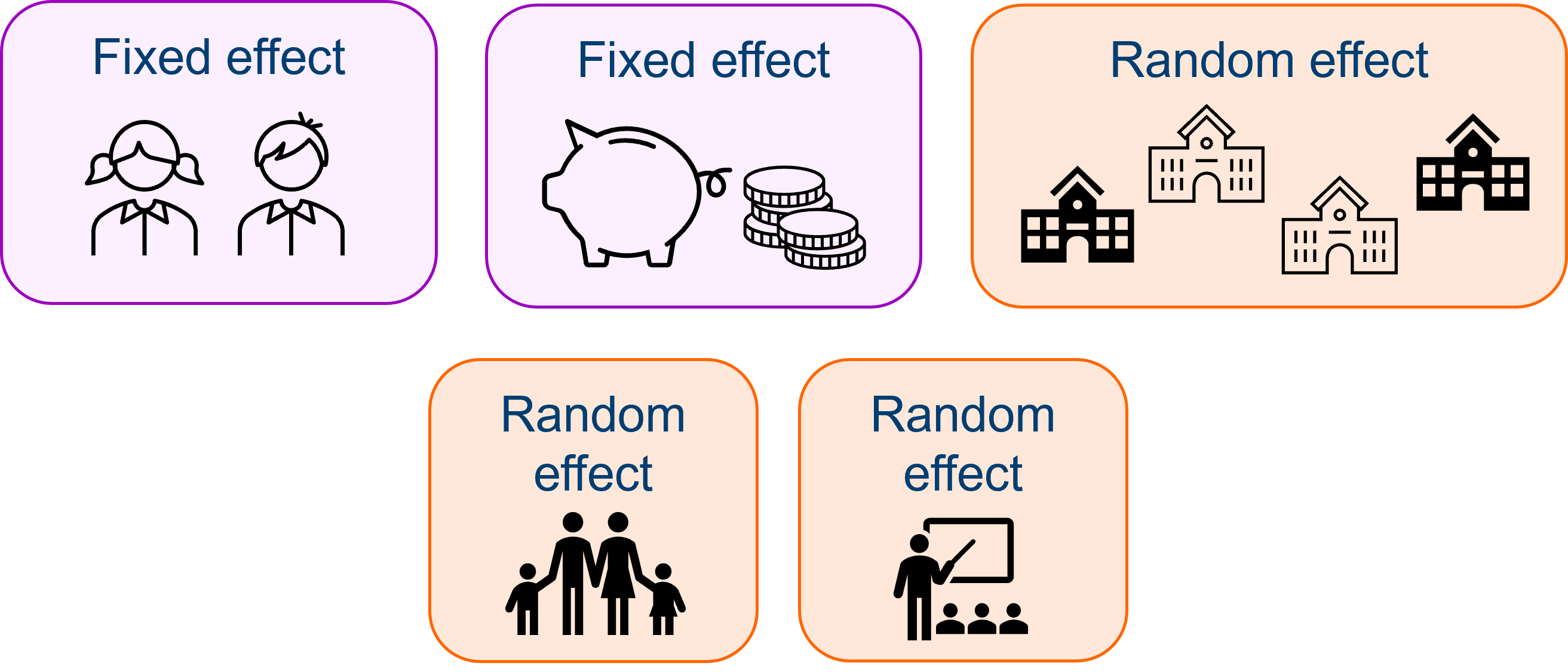 We also have two possible “hidden” random effects in this dataset, however.
The first is classroom. If the final year students are grouped into more than one class within each school, then they have been further “clustered”. Students from the same class share a teacher, and thus will be more similar to one another than to students in another class, even within the same school.
The classroom variable would in fact be “nested” inside the school variable - more on nested variables in later sections of this course.
Our other possible hidden variable is family. If siblings have been included in the study, they will share an identical SES score, because this has been derived from the parent(s) rather than the students themselves. Siblings are, in this context, technical replicates! One way to deal with this is to simply remove siblings from the study; or, if there are enough sibling pairs to warrant it, we could also treat family as a random effect.
4.2.2 Ferns
Level:
A plant scientist is investigating how light intensity affects the growth rate of young fern seedlings.
He cultivates 240 seedlings in total in the greenhouse, split across ten trays (24 seedlings in each). Each tray receives one of three different light intensities, which can be varied by changing the settings on purpose-built growlights.
The height of each seedling is then measured repeatedly at five different time points (days 1, 3, 5, 7 and 9).
What are our variables? What’s the relationship we’re interested in, and which of the variables (if any) should be treated as random effects?
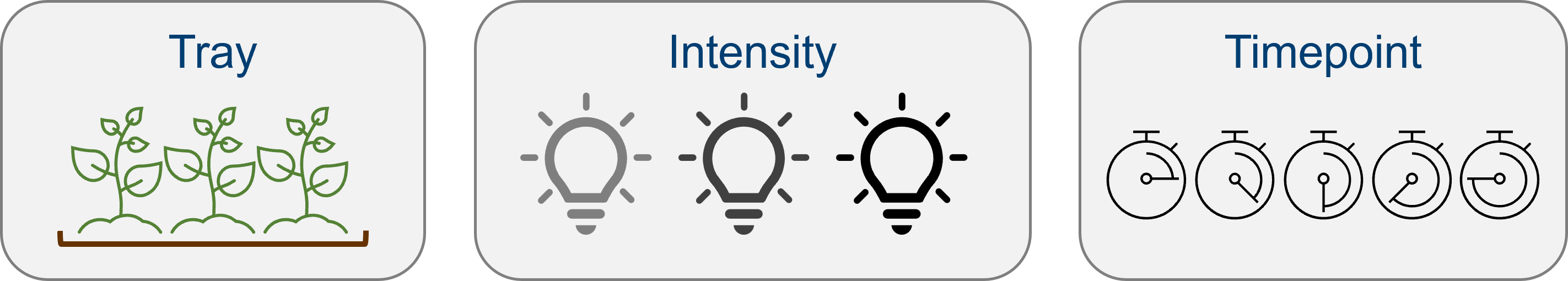
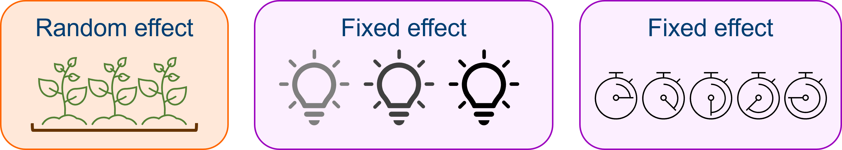
There are four things here that vary: tray, light intensity, timepoint and height.
We’re interested in the relationship between growth rate and light intensity. This makes our first two predictor variables easier to decide about:
 The variable
 tray is a random effect here. We are not interested in differences between these 10 particular trays that we’ve grouped our seedlings into, but we do need to recognise the non-independence created by these natural clusters - particularly because we’ve applied the “treatment” (changes in light intensity) to entire trays, rather than to individual seedlings.
In contrast, light intensity - though a categorical variable - is a fixed effect. We are specifically interested in comparing across the three light intensity levels, so we don’t want to share information between them; we want fixed estimates of the differences between the group means here.
Perhaps the trickiest variable to decide about is time. Sometimes, we will want to treat time as a random effect in mixed effects models. And we have enough timepoints to satisfy the requirement for 5+ levels in this dataset.
But in this instance, where we are looking at growth rate, we have a good reason to believe that time is an important predictor variable, that may have an interesting interaction with light intensity.
Further, our particular levels of time - the specific days that we have measured - are not necessarily exchangeable, nor do we necessarily want to share information between these levels.
In this case, then, time would probably be best treated as a fixed rather than random effect.
However, if we were not measuring a response variable that changes over time (like growth), that might change. If, for instance, we were investigating the relationship between light intensity and chlorophyll production in adult plants, then measuring across different time points would be a case of technical replication instead, and time would be best treated as a random effect. The research question is key in making this decision.
4.2.3 Wolves
Level:
An ecologist is conducting a study to demonstrate how the presence of wolves in US national parks predicts the likelihood of flooding. For six different national parks across the country that contain rivers, they record the estimated wolf population, and the average number of centimetres by which the major river in the park overflows its banks, for the last 10 years - for a total of 60 observations.
What’s the relationship of interest? Is our total n really 60?
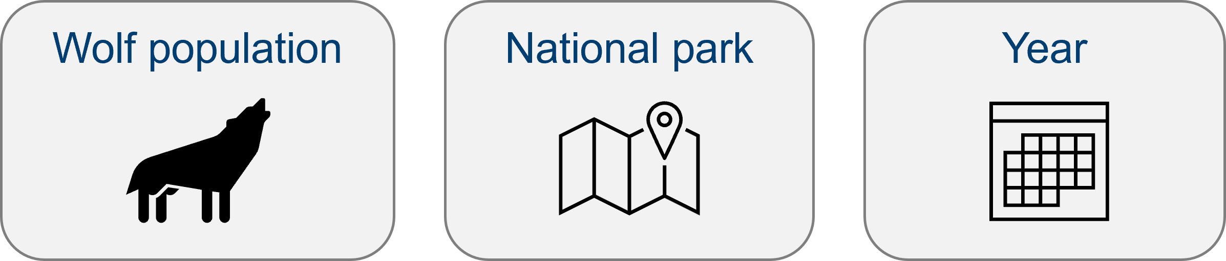
Though we have 60 observations, it would of course be a case of pseudoreplication if we failed to understand the clustering within these data.
We have four things that vary: wolf population, flood depth, national park and year.
With flood depth as our response variable, we already know how to treat that. And by now, you’ve hopefully got the pattern that our continuous effect of interest wolf population will always have to be a fixed effect.
 But there’s also
 year and national park to contend with, and here, we likely want to treat both as random effects.
We have measured across several national parks, and over a 10 year period, in order to give us a large enough dataset for sufficient statistical power - these are technical replicates. But from a theoretical standpoint, the exact years and the exact parks that we’ve measured from, probably aren’t that relevant. It’s fine if we share information across these different levels.
Of course, you might know more about ecology than me, and have a good reason to believe that the exact years do matter - that perhaps something fundamental in the relationship between flood depth ~ wolf population really does vary with year in a meaningful way. But given that our research question does not focus on change over time, both year and national park would be best treated as random effects given the information we currently have.
4.3 Summary
- A model with both fixed and random effects is referred to as a mixed effects model
- Random effects are categorical variables, with 5+ levels, that represent non-independent “clusters” or “groups” within the data
- Random effects are estimated by sharing information across levels/groups, which are typically chosen “at random” from a larger set of exchangeable levels
- Whether a variable should be treated as a random effect depends both on the nature of the variable, and also the research question