6 Preparing data
After this section you should be able to:
- Recognise the importance of organising your files and folders when starting a bioinformatic analysis.
- Use the command line to create the directories that will be used for your analysis.
- Investigate the content of sequencing FASTQ files.
- Recognise the importance of metadata for data interpretation and discuss its relevance for pathogen surveillance.
- Access and download genomes from public databases.
6.1 Data overview
In the examples used throughout these materials we will use sequencing data for the cholera bacterium Vibrio cholerae. The material was obtained from cultured samples, so each sequencing library was prepared from DNA extracted from a single plate colony. We have two datasets, as summarised below.
This dataset is used for the examples shown in the main text. These data are not available for download (see dataset 2 instead).
- Number of samples: 10
- Origin: unspecified country (due to privacy concerns), but all patients showed AWD symptoms, suspected to be due to a local cholera outbreak.
- Sample preparation: stool samples were collected and used for plate culture in media appropriate to grow Vibrio species; DNA was prepared using the Zymobiomics Fungal/Bacterial DNA miniprep kit; ONT library preparation and barcoding were done using standard ONT kits.
- Sequencing platform: MinION
- Basecalling: Guppy version 6 in “fast” mode
This dataset is used for the exercises and can be downloaded (see Setup & Data). This is part of a public dataset from Ambroise et al. 2003 (see publication for further details).
- Number of samples: 5
- Origin: samples from cholera patients from the Democratic Republic of the Congo.
- Sample preparation: stool samples were collected and used for plate culture in media appropriate for growing Vibrio species; ONT library preparation and barcoding were done using standard kits.
- Sequencing platform: MinION, using FLO-MIN112 (R10 version) flowcells.
- Basecalling: Guppy version 6 in “fast” mode (this information is not actually specified in the manuscript, but we are making this assumption just as an example).
If you are attending one of our workshops that includes lab training, you can use the data produced during the workshop in the exercises.
6.2 Setting up directories and preparing files
For convenience and reproducibility of any bioinformatic analysis, it is good practice to set up several directories before starting your analysis. It is also convenient to download any required files from public databases, such as reference genomes.
You can do this from your file browser or using the command line. We recommend starting with a new directory that will be used to store all the data and scripts used during the analysis. For example, let’s say we are working from a directory in our Documents called awd_workshop. Here are some recommended directories that you should create inside it:
data- for storing raw sequencing data (fastq files).scripts- for storing all scripts for running analysis at different stages.results- for storing results of the pipeline.reports- for storing reports of the analysis.resources- for storing files from public repositories, such as reference genomes and other databases we will require during our analysis.
If you’re attending one of our live workshops, we’ve already prepared the data for you to save time in downloading and preparing the files. However, you can read this section to understand where the data came from.
From the command line, you can create directories using the command mkdir. In our example, we will be working from our Documents folder, which is located in ~/Documents/ (remember that ~ is a shortcut to your home directory).
We start by moving into that directory:
cd ~/DocumentsAnd then we create a folder for our project. We call this folder awd_workshop:
mkdir awd_workshopWe can then move into that folder using cd again:
cd awd_workshopFinally, we create all the sub-directories to save our different pieces of data:
# create several directories simultaneously with a single command
mkdir data scripts results resources reports
6.3 Sequencing files
Our bioinformatics analysis will start by first looking at the FASTQ files generated by the basecalling software called Guppy. This software converts the Nanopore electrical signal to sequence calls and stores the results in a directory named fastq_pass, which contains a subdirectory for each sample barcode used.
We have copied/pasted the fastq_pass folder from Guppy into our data directory simply using our file browser. We can use the command ls to view what’s inside it:
ls data/fastq_passbarcode25 barcode27 barcode29 barcode31 barcode33
barcode26 barcode28 barcode30 barcode32 barcode34In our example, we had 10 samples with the barcodes shown (yours might look different).
If you wanted to quickly look at how many reads you have in each file, you could use some command line tricks:
- first combine all the FASTQ files from a barcode using
zcat(we use thez*variant of thecatcommand because our files are compressed) - pipe the output to the
wc -lto count the number of lines in the combined files - then divide that number by 4, because each sequence is represented in 4 lines in FASTQ files
For example, for barcode25 we could do:
zcat data/fastq_pass/barcode25/*.fastq.gz | wc -l484416If we divide that value by 4, we can determine that we have 121,104 reads in this sample.
The following code is more advanced, but it allows us to determine how many reads we have in each barcode without having to type each command individually. Instead, we use a for loop to automatically perform our task of counting reads for each barcode.
If you feel confortable using the command line, you can try it out.
for barcode in data/fastq_pass/*
do
  # count total lines in all files within a barcode folder
  nlines=$(zcat $barcode/* | wc -l)

  # divide the value by 4 (each sequence is represented in 4 lines in FASTQ files)
  nreads=$(( $nlines / 4 ))

  # print the result
  echo "Reads in ${barcode}: ${nreads}"
done
Reads in data/fastq_pass/barcode25: 121104
Reads in data/fastq_pass/barcode26: 202685
Reads in data/fastq_pass/barcode27: 247162
Reads in data/fastq_pass/barcode28: 262453
Reads in data/fastq_pass/barcode29: 157356
Reads in data/fastq_pass/barcode30: 286582
Reads in data/fastq_pass/barcode31: 187090
Reads in data/fastq_pass/barcode32: 120555
Reads in data/fastq_pass/barcode33: 121991
Reads in data/fastq_pass/barcode34: 102589To learn more about for loops see our Unix course materials.
6.4 Metadata
Having metadata (data about our raw FASTQ files) is important in order to have a clear understanding on how the samples and raw data were generated. Two key pieces of information for genomic surveillance are the date of sample collection and the geographic location of that sample. This information can be used to understand which strains of a pathogen are circulating in an area at any given time. Information like the protocol used for preparing the samples (e.g. metagenomic or culture-based) and the sequencing platform used (Illumina or ONT) are also crucial for the bioinformatic analysis steps. Metadata is thus important for downstream analyses, results interpretation and reporting.
Privacy concerns need to be considered when collecting and storing sensitive data. However, it should be noted that sensitive data can still be collected, even if it is not shared publicly. Such sensitive information may still be useful for the relevant public health authorities, who may use that sensitive information for a finer analysis of the data. For example, epidemiological analysis will require individual-level metadata (“person, place, time”) to be available, in order to track the dynamics of transmission within a community.
The most general advice when it comes to metadata collection is: record as much information about each sample as possible!
Some of this information can be stored in a CSV file, created with a spreadsheet software such as Excel.
6.5 Public genomes
In our example, we are working with cultured samples of the Vibrio cholerae bacteria, the causative pathogen of the cholera disease, of which AWD is a major symptom. Therefore, we have downloaded public genomes for this pathogen, which will later be used to understand how our strains relate to others previously sequenced.
There are many complete genomes available for V. cholerae, which can be downloaded from the NCBI public database. The first full genome was published in 2000 from the clinical isolate N16961, which belongs to serogroup O1, serotype Inaba, biotype El Tor. This is a typical strain from the current pandemic, often referred to as ‘7PET’ (7th pandemic El Tor).
The Vibriowatch website (which we will detail more about in a later chapter) also provides a set of 17 ‘reference genomes’, 14 of which belong to the current pandemic (7PET) lineages. Their reference genomes are named as ‘Wi_Tj’ where ‘W’ stands for a Wave and ‘i’ is its number, and ‘T’ stands for Transmission event and ‘j’ its number. For instance, a W1_T1 strain means “wave one transmission event one”.
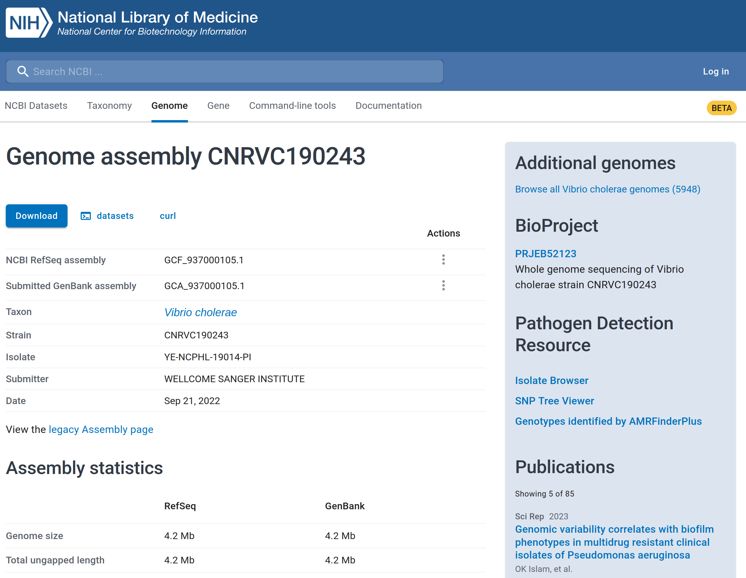
For example, we can look at a public strain related to ‘W3_T13’, associated with a cholera outbreak in Yemen in 2019. This sample is available from the following link: https://www.ncbi.nlm.nih.gov/datasets/genome/GCF_937000105.1/.
From the link above you can see information about the genome assembly of this strain, as shown below. The assembly is complete with 99.69% of the genome recovered.
In that same page, you will see a “Download” button. When you click that button, the pop-up window will be displayed as illustrated in the image below.
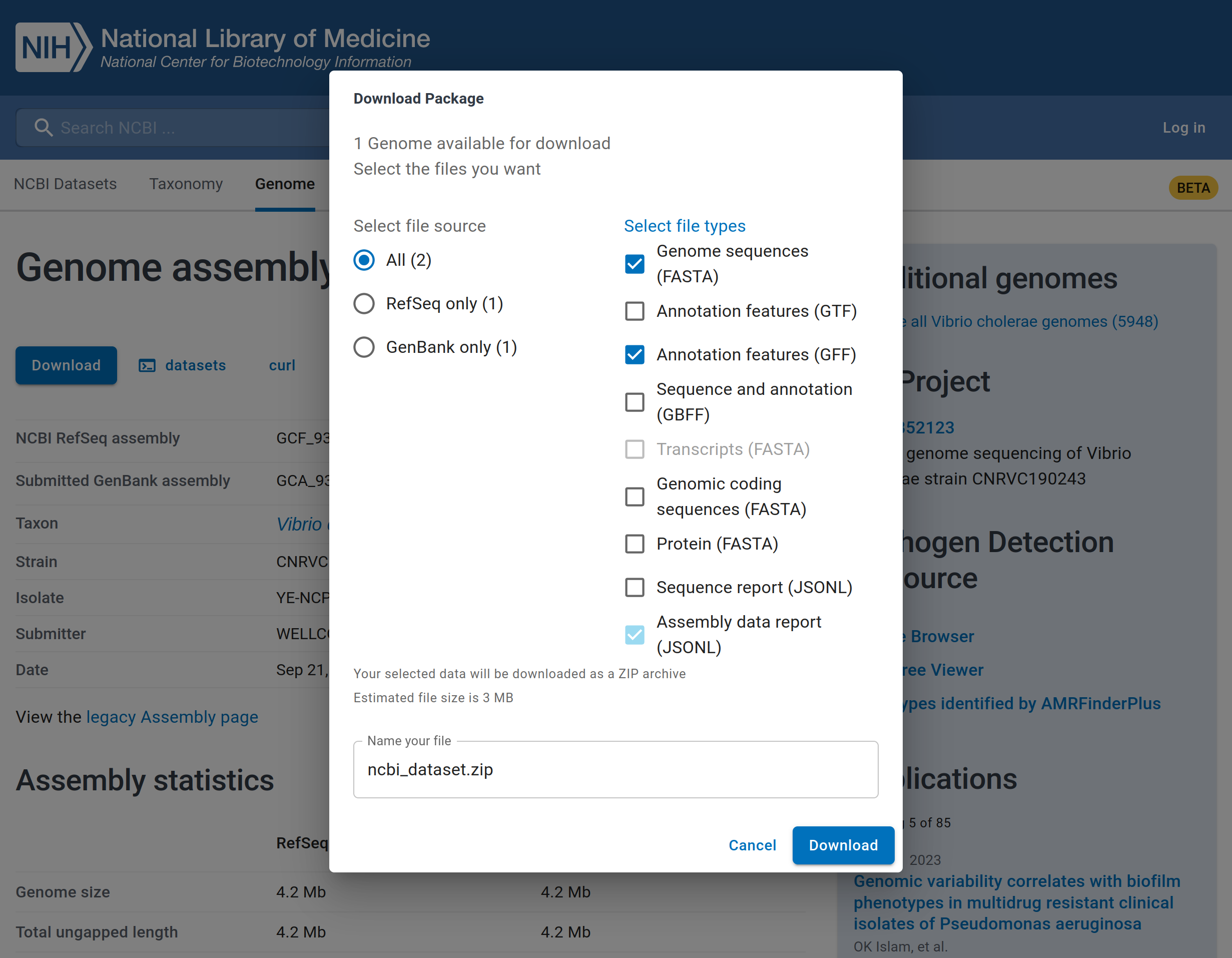
The reference genome sequence can be selected by ticking ‘Genome sequences (FASTA)’ and the gene annotation by ticking ‘Annotation features (GFF)’ formats. You can change the name of the file that will be downloaded and finally, click the ‘Download’ button to download the reference genome assembly.
The downloaded file is compressed as a Zip file, which you can uncompress and copy the files to your project folder. For this workshop, we have downloaded 31 samples and saved them in the directory resources/vibrio_genomes. We will later use these genomes for our phylogenetic analysis.
We can check all our genomes with the ls command:
ls resources/vibrio_genomesGCF_004328575.1_ASM432857v1_genomic.fna GCF_013462495.1_ASM1346249v1_genomic.gff GCF_021431865.1_ASM2143186v1_genomic.fna
GCF_004328575.1_ASM432857v1_genomic.gff GCF_015482825.1_ASM1548282v1_genomic.fna GCF_021431865.1_ASM2143186v1_genomic.gff
GCF_009763665.1_ASM976366v1_genomic.fna GCF_015482825.1_ASM1548282v1_genomic.gff GCF_021431945.1_ASM2143194v1_genomic.fna
GCF_009763665.1_ASM976366v1_genomic.gff GCF_017948285.1_ASM1794828v1_genomic.fna GCF_021431945.1_ASM2143194v1_genomic.gff
... more output ommitted ...You can see that for each sample we have an .fna file (FASTA format) and a .gff file (GFF format). See Section 5.2 for a recap of these file formats.
For each of these samples we also obtained some metadata, which is stored in a tab-delimited (TSV) file:
head resources/vibrio_genomes/public_genomes_metadata.tsvname display_name clade mlst biotype serogroup
GCF_009763665.1_ASM976366v1_genomic GCF_009763665.1 Env_Sewage 1258 NA NA
GCF_023169825.1_ASM2316982v1_genomic GCF_023169825.1 Env_Sewage 555 NA NA
GCF_937000115.1_CNRVC190247_genomic GCF_937000115.1 Env_Sewage 555 NA NA
GCF_004328575.1_ASM432857v1_genomic GCF_004328575.1 M66 178 NA NA
GCF_019458465.1_ASM1945846v1_genomic GCF_019458465.1 M66 1257 NA NA
GCF_021431945.1_ASM2143194v1_genomic GCF_021431945.1 M66 1092 NA NA
GCF_026013235.1_ASM2601323v1_genomic GCF_026013235.1 M66 167 NA NA
GCF_009763945.1_ASM976394v1_genomic GCF_009763945.1 W1_T2 69 O1 El Tor O1
GCF_013085075.1_ASM1308507v1_genomic GCF_013085075.1 W1_T2 69 O1 El Tor O1This provides information for each sample, which we will discuss in later sections.
6.6 Summary
- Proper file and folder organization ensures clarity, reproducibility, and efficiency throughout your bioinformatic analysis.
- Organising files by project, and creating directories for data, scripts and results helps prevent data mix-ups and confusion.
- Command line tools like
mkdirallow you to create directory structures efficiently. - Directories should have meaningful names to reflect their contents and purpose.
- FASTQ files containing the raw sequencing data, can be quickly investigated using standard command line tools, for example to count how many reads are available.
- Metadata provides context to biological data, including sample information, experimental conditions, and data sources.
- In pathogen surveillance, metadata helps trace the origin and characteristics of samples, aiding outbreak investigation.
- Public genomic databases like NCBI and platforms such as Pathogenwatch provide a vast collection of sequenced genomes.
- Access to these resources allows researchers to retrieve reference genomes for comparative analyses.